File Format of XGC Mesh Files
XGC requires three input files to set up its triangular solver mesh:
A file containing the cylindrical coordinates R and Z of the mesh vertices (the “node” file).
A file containing the triangle connectivity of the vertices (the “ele” file).
A file containing the flux-surface connectivity of the vertices (the “flx” file).
The following paragraphs describes the file format of those files. Stellarator simulations with XGC-S require other mesh files described in the last paragraph.
The “node” File
The “node” file starts with a header line that contains the number of vertices of the mesh, dimension (must be 2), number of attributes and number of boundary markers (0 or 1). The information is in the following format:
<number of vertices> <dimension> <number of attributes> <number of boundary markers>
XGC only supports:
dimension = 2
number of attributes = 0
number of boundary markers = 1
The header line in the “node” file should look like this
<number of vertices> 2 0 1
Each of the following lines contains the R and Z coordinates of the mesh vertices, e.g.:
181162  2  0  1
1 1.218645 -1.363000 0
2 1.216197 -1.363000 0
3 1.220985 -1.363000 0
4 1.218374 -1.360182 0
5 1.220244 -1.360709 0
[...]
The vertex data is arranged in four columns. The first column is the vertex index. The second and third column are the R and Z coordinates, and the last column indicates whether the vertex is on the wall curve (1) or not (0).
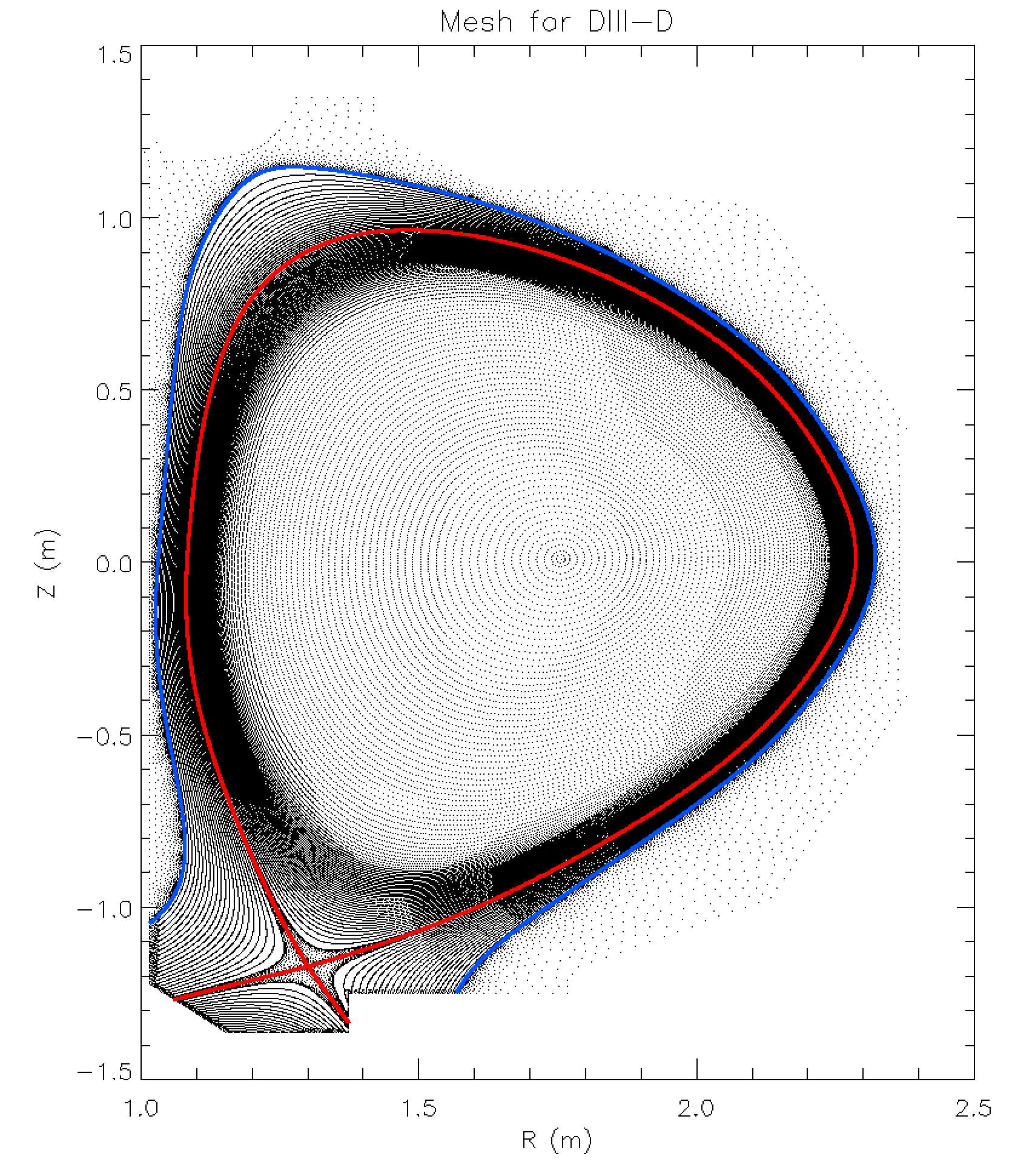
Fig. 1: Example of an XGC mesh. There are four distinct regions, i) the closed flux-surface region (core), ii) the scrape-off layer (SOL), iii) the private flux region, and iv) the unstructured mesh region (outside the blue surface). The separatrix, which includes the X-point and separates core, SOL and private region, is shown in red. There are cases with two X-points and two separatrices within the wall curve. In those cases, there is also a second private region.
The “ele” file
The “ele” file contains the triangle connectivity of the mesh. The header line in the file contains the number of triangles, nodes per triangle and number of attributes. The information is in the following format:
<number of triangles> <nodes per triangle> <number of attributes>
XGC only supports:
nodes per triangle = 3
number of attributes = 0
The header line in the “ele” file should look like this
<number of triangles> 3 0
Each of the following lines lists the triangle index and the indices of the three vertices of the triangle, e.g.:
361725        3        0
   1      2      1      4
   2      5      1      3
   3      1      5      4
   4      2      7      6
   5      2      8      7
   6      8      2      4
   7     10      3      9
   [...]
The “flx” file
Most vertices in XGC meshes are not really unstructured, but are aligned on a set of surfaces of constant poloidal magnetic flux (flux-surfaces or flux-curves). The minority of vertices is really unstructured. In this sense, XGC meshes are divided into two regions, the field-aligned and unstructured regions. The two regions are separated by the blue flux-surface in Fig. 1. Around the X-point and where flux-surfaces intersect with the wall curve, additional vertices that are not field-aligned have to be added to generate high-quality meshes. Those vertices are called “non-aligned vertices” in the remainder of this section. Fig. 2 shoes an example of those non-aligned vertices.
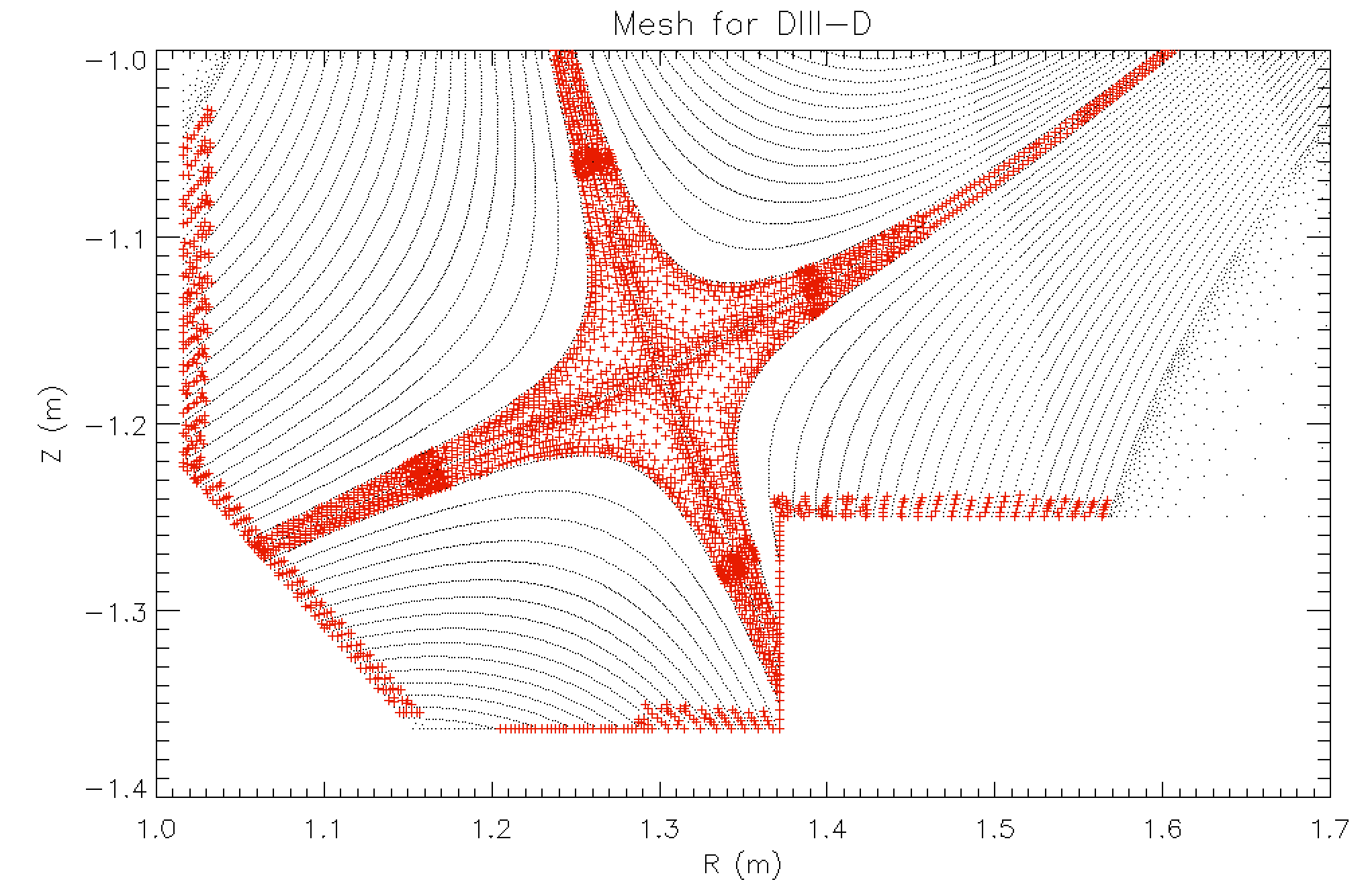
Fig. 2: Nonaligned vertices are shown in red, field-aligned vertices and unstructured vertices are shown in black. The non-aligned vertices are all in the region that is otherwise filled with field-aligned mesh (inside the blue surface in Fig. 1).
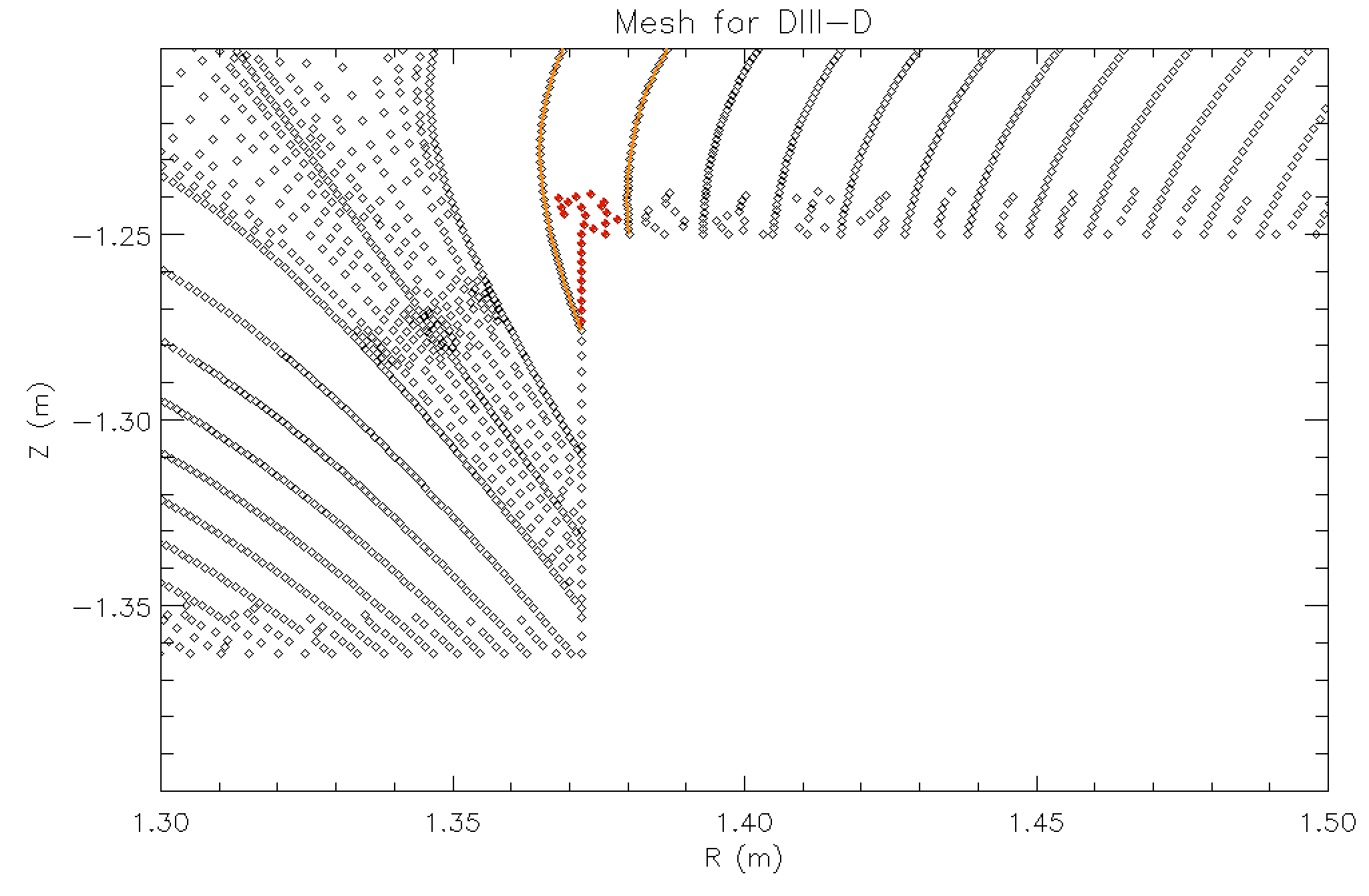
Simply speaking, flux-surface averages <A> in XGC are computed by calculating the mean of A over the vertices on the same flux-surface. In many situations, it is necessary to know the value of <A> on each vertex of the mesh. This value is readily obtained for all field-aligned vertices. The value of <A> on the non-aligned vertices, on the other hand, is obtained through interpolation from the field-aligned vertices. In XGC, linear interpolation is used, which requires knowledge of the two flux-surfaces between which each non-aligned vertex lies. Fig. 3 shows an example. Two adjacent flux surfaces are shown in orange, and the non-aligned vertices between them are shown in red.
The “flx” file contains lists of vertices that are on the same flux-surface, the two flux-surfaces associated with each of the non-aligned vertices, and some other information about the mesh structure.
1
1920   -1
93 23 16  0
94 -1
   1   11   21   29
 69137
 70218  70221  70222  70223 [...]
 72375  72376  72377  72378 [...]
 75593  75597  75598  75599 [...]
[...]
-1
3893
11131
106 107
10822
106 107
10825
106 107
 10532
-1
The first line is the number of separatrices/X-points in the mesh (currently a maximum of two is supported. The second line contains the indices of the X-point vertices. The third line is the number of flux-surfaces in the core, the SOL, the lower private region and the upper private region (if it exists). The fourth line contains the indices of the separatrix flux-surfaces. The fifth line contains the number of vertices on each flux-surface. The following lines until the first line with -1 are lists of indices of vertices. The length of each line is given by the numbers in line 5. The line after the first -1 is the number of non-aligned vertices. Finally, the following lines until the second -1 give the index of each non-aligned vertex and the indices of the two associated flux-surfaces.
Stellarator Mesh Files
The “node” and “ele” files
The “node” and “ele” files are the same for XGC-S simulations as for tokamak XGC simulations. However, in stellarator geometry each plane has a different mesh so each plane has its own “node” and “ele” files. Moreover, for XGC-S the “node” file has 2 attributes instead of 0 and six columns where the 2 extra (column 4 and 5) represent normalized minor radius and poloidal angle in VMEC or PEST coordinates. The last column (0000 or 0001) indicates whether the node is on the boundary curve (last closed flux-surface) or not. The \(R\) and \(Z\) values are in meters.
      9629   2  2  1
   1       0.59531987E+001   0.00000000E+000   0.00000000E+000   0.00000000E+000   0000
   2       0.59568025E+001   0.00000000E+000   0.15079365E-001   0.00000000E+000   0000
   3       0.59557115E+001   0.98804646E-002   0.15079365E-001   0.78539819E+000   0000
   4       0.59531048E+001   0.13988747E-001   0.15079365E-001   0.15707964E+001   0000
   5       0.59505910E+001   0.98972425E-002   0.15079365E-001   0.23561946E+001   0000
[...]
i          R                 Z                 (psi/psi_a)^(1/2) Poloidal angle    Boundary flag
[...]
9627       0.61620301E+001  -0.50909058E-001   0.95000000E+000   0.62203536E+001   0001
9628       0.61627405E+001  -0.33957567E-001   0.95000000E+000   0.62412976E+001   0001
9629       0.61631671E+001  -0.16984191E-001   0.95000000E+000   0.62622415E+001   0001
Example of a “node” file for XGC-S.
The “node” and “ele” files can be viewed with Triangle.
> /PATH_TO_TRIANGLE/triangle/showme w7x_test_0011.node
|
|
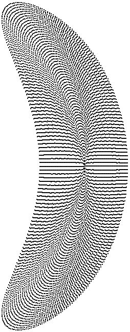
Fig. 4: Example of two W7-X “node” files displayed with “Show Me” in Triangle.
The “grid” file
The “grid” file is used in XGC-S instead of the “flx” file in tokamak XGC. The header line contains the total number of discretized flux-surfaces, the number of mesh vertices on the surface per toroidal cross-section and normalized poloidal flux (label) of the surface. The other lines contain three columns with the index of the flux-surface, the number of mesh vertices on the surface per toroidal cross-section and normalized poloidal flux (label) of the surface.
64           1              0.000000000000E+000
 2           8              0.227387251197E-003
 3          12              0.909549004787E-003
 4          16              0.204648526077E-002
 5          20              0.363819601915E-002
[...]
i          N_{node}         psi/psi_a
[...]
62         288              0.846107961703E+000
63         292              0.874076593600E+000
64         300              0.902500000000E+000
Example of a “grid” file for XGC-S.
The “iota” file
The “iota” file is read by XGC-S and must be present for a simulation to work, but it is not used by the code at the moment. The file contains four columns: index of the normalized poloidal flux (1 - 10000), normalized minor radius (i.e. square root of normalized poloidal flux), normalized poloidal flux (label), rotational transform (iota).
    1      0.000000000000E+000        0.000000000000E+000    0.854068450766E+000
    2      0.100010001000E-003        0.100020003000E-007    0.854068451590E+000
    3      0.200020002000E-003        0.400080012002E-007    0.854068454064E+000
    4      0.300030003000E-003        0.900180027004E-007    0.854068458187E+000
    5      0.400040004000E-003        0.160032004801E-006    0.854068463958E+000
[...]
i          (psi/psi_a)^(1/2)          psi/psi_a              iota
[...]
 9998      0.999799979998E+000        0.999600000004E+000    0.939869651277E+000
 9999      0.999899989999E+000        0.999799990000E+000    0.939887666419E+000
10000      0.100000000000E+001        0.100000000000E+001    0.939905683859E+000
Example of a “iota” file for XGC-S.
The “dat” files
The “dat” files contain magnetic field data in cylindrical coordinates and each plane has its own “dat” file. Assuming that VMEC2XGC2 has been run with the flag -format 2, the “dat” files have the following format. There are two header lines starting with # (the header lines are the same in all “dat” files of a mesh).
The first line contains 4 values: The first 2 represent the number of number of grid points in \(R\) and \(Z\). The 3rd value is the number of toroidal cross-section. These numbers are set by the input -spline and -nv to VMEC2XGC2. The 4th value is the toroidal periodicity from the VMEC file or torus wedge number for a tokamak.
The second header line also contains 4 values: The first 2 are \(R_\min\) and \(R_\max\) whereas the last 2 are \(Z_\min\) and \(Z_\max\).
The remaining lines have eight columns: Column 1 and 2 represent index in \(R\) and \(Z\). Column 3 is the normalized poloidal flux. Column 4 and 5 contain the poloidal angle in VMEC and PEST coordinates (not used in XGC-S). Column 6, 7 and 8 are the magnetic field components \(B_R\), \(B_\varphi\) and \(B_z\).
#  100  100   37    5
#   0.46119258E+001   0.61739443E+001  -0.89249210E+000   0.89249210E+000
0001        0001         0.10217834E+002   0.33235219E+001   0.10000000E+002   0.49319421E+000   0.26404557E+001   0.12471970E+001
0002        0001         0.92666642E+001   0.33260341E+001   0.10000000E+002   0.49935416E+000   0.26493748E+001   0.12444712E+001
0003        0001         0.98682945E+001   0.33286185E+001   0.10000000E+002   0.50564983E+000   0.26582892E+001   0.12416419E+001
0004        0001         0.82809115E+001   0.33312826E+001   0.10000000E+002   0.51212162E+000   0.26671979E+001   0.12386898E+001
0005        0001         0.95277351E+001   0.33340292E+001   0.10000000E+002   0.51876230E+000   0.26761009E+001   0.12356130E+001
[...]
i_R         i_Z          psi/psi_a         VMEC angle        PEST angle        B_R               B_{varphi}        B_Z
[...]
0098        0100         0.32156580E+001   0.61496809E+000   0.10000000E+002  -0.39181317E+000   0.28231810E+001   0.60535254E+000
0099        0100         0.33071149E+001   0.59809262E+000   0.10000000E+002  -0.38284840E+000   0.28253084E+001   0.60734149E+000
0100        0100         0.34422752E+001   0.58183519E+000   0.10000000E+002  -0.37408281E+000   0.28276989E+001   0.60921698E+000
Example of a “dat” file for XGC-S.
The “flux” and “mag” files
There are one “flux” file and three “mag” files for each plane. The “flux” files contain the normalized poloidal flux (label) \(\psi\) spline coefficients and the “mag” files the corresponding \(B_R\), \(B_\varphi\) and \(B_Z\) spline coefficients. These are files in binary format obtained by running the spline coefficients tool on the “dat” files.