Generating Meshes for XGC Simulations¶

XGC Simulations Rely on Unstructured Triangular Configuration Space Meshes¶

Most gyrokinetic codes use flux-coordinates, i.e., coordinates in which the field line pitch is constant on a flux-surface, because they are the natural choice for separating motion and spatial scales parallel and perpendicular to the magnetic field. Flux-coordinates enable simulations with low resolution along the magnetic field B for perturbations with low parallel wavenumber $k_\parallel=\frac{\mathbf{B}}{|B|}\cdot\mathbf{k}$. However, the metric of flux-coordinates has singularities on the magnetic axis and the separatrix. This is a problem for whole-volume simulations.

XGC computes particle trajectories in right-handed cylindrical coordinates $(R,\varphi,Z)$ to avoid coordinate singularities. This approach is good for whole-volume simulations from the magnetic axis to the material wall. In cylindrical coordinates, general unstructured meshes would require very high resolution in all three dimensions. But for simulation of tokamak and stellarator turbulence, which is characterized by low $k_\parallel$ and high perpendicular wavenumbers ($k_\perp \rho_s \sim 1$), it is still possible to use reduced toroidal resolution similar to flux-coordinates. This is achieved by aligning the mesh vertices on a finite number of magnetic flux-surfaces placed such that they are approximately aligned with the magnetic field. See the following sections for more details.

References:

Configuration Space Discretization¶

Toroidal Discretization¶

In the toroidal ($\varphi$) direction, configuration space is discretized on a uniform toroidal angle grid of size $N_\varphi$. That is, the topological torus is divided into $N_\varphi$ sections.

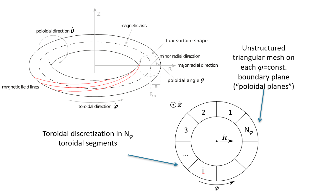
Radial-Poloidal Plane¶

On the radial-poloidal ($\varphi=\text{const.}$) plane, configuration space is discretized using unstructured triangle meshes with linear finite elements. That is, there is an unstructured mesh on each boundary between adjacent toroidal sections. In axisymmetric magnetic confinement devices (i.e., tokamaks), those meshes are identical on each radial-poloidal plane. In stellarator geometry, each plane has a different mesh. However, the planar meshes are not entirely unstructured. Most vertices are placed on a finite number of flux-surfaces in an approximately field-aligned way. This means that a magnetic field-line starting from a vertex on plane $\varphi_i=2\pi i/N_\varphi$ intersects plane $\varphi_{i+1}$ at or very close to another vertex. The approximate field-alignment of the XGC meshes enables simulation of strongly anisotropic turbulence (low $k_\parallel$, high $k_\perp$) with low toroidal resolution similar to gyrokinetic codes using flux-coordinates, but without the associated coordinate singularities [see R. Hager et al., Physics of Plasmas 29, 112308 (2022)].

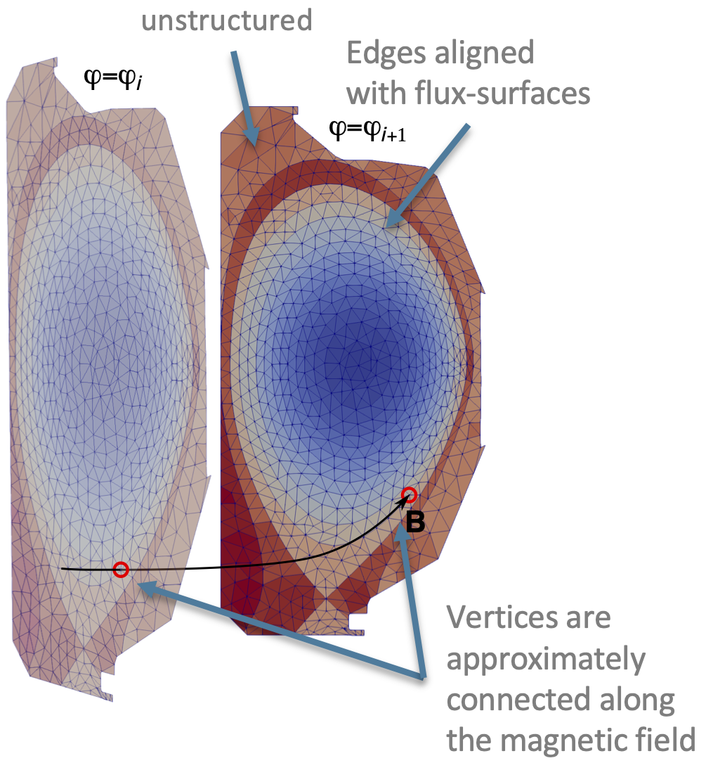
Illustration of approximate field alignment¶

Typical Mesh Size¶

Mesh size in radial-poloidal plane: ~1-4 mm
Device size: $\sim 1 \text{m} \rightarrow N_n \sim 10^{4}\text{-}10^{6}$ vertices per radial-poloidal plane
$\sim 10^4$ marker particles per vertex
DIII-D size simulation
- Axisymmetric ($N_\varphi=1$): $\sim 30,000-50,000$ vertices, $\sim 500\cdot 10^6$ particles/species
- Non-axisymmetric ($N_\varphi \sim 32$): $\sim 5 \cdot 10^6$ vertices, $\sim 50 \cdot 10^9$ particles/species
ITER size simulation
- Non-axisymmetric ($N_\varphi=32$): $\sim 32 \cdot 10^6$ vertices, $>320\cdot 10^9$ particles/species

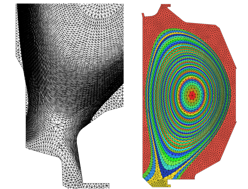
C-Mod and D3D Meshes¶

The Tokamak Modeling and Meshing Software (TOMMS)¶

Meshes for XGC simulations are generated using the Tokamak Modeling and Meshing Software (TOMMS) developed at the Scientific Computation Research Center (SCOREC) at Rensselaer Polytechnic Institute (RPI) in collaboration with Simmetrix. The meshing tool is installed on the PPPL cluster Portal (portal.pppl.gov) and actively maintained. Installation on other resources is possible but requires a license for the Simmetrix products SimModSuite and SimModeler.

TOMMS can be run as a command line tool or with a Graphical User Interface (GUI) available in Simmetrix SimModeler. TONMS produces high quality meshes and has the following key features

Triangular 2D mesh of a poloidal plane with field-following vertices for the user-defined region of a tokamak.

Flux-surfaces with one element deep mesh (i.e. one element between two adjacent flux surface).

Unstructured meshes for undefined parts of the scrape-off layer and private flux regions.

The code supports tokamak geometries with multiple X-points.

We rely on feedback from users to continually improve this tool. If you experience problems, contact Robert Hager (rhager@pppl.gov) or Seung-Hoe Ku (sku@pppl.gov) and/or open a Github issue at https://github.com/SCOREC/Fusion_Public.

Environment Setup on Portal¶

TOMMS is available on portal.pppl.gov. To set up your shell environment for running TOMMS, just run

> source /p/xgc/Software/bin/setup_tomms_meshgen

If you maintain your own installation of TOMMS, remember to set the number of OpenMP threads to 1:

> export OMP_NUM_THREADS=1

To run the command-line version of TOMMS:

> tomms_meshgen

For the GUI:

> simmodeler

In SimModeler, select the “Fusion” tab.

TOMMS Documentation and Support¶

A user guide and description of every control parameter can be found on the following public pages:
- User Guide
- Input Parameters
Sample test cases with working input files (xgc_mesh_in) can be found in the following public directory:
- Meshing Examples
- The cases already contain a working input file (xgc_mesh_in). The user needs to set up the environment and call the TOMMS executable as described above.

A Step-by-step Guide to XGC Tokamak Mesh Generation¶

Collect the Required Input Data¶

Certain input files are mandatory, others are optional. At the very least, the following two input files are required:

Magnetic equilibrium in
- EFIT geqdsk format, or
- XGC-eqd format: generated with efit2eqd included in the XGC repository; works only for cases without X-point, e.g. Cyclone).
- The resolution of the EFIT geqdsk/eqd files should be at least 256x256.
Input file with meshing parameters (default name: xgc_mesh_in).
- In the SimModeler GUI, meshing parameters can be manually entered or read from file.

Optional input files are:

Ion temperature profiles as function of the normalized poloidal magnetic flux $\psi_N=\frac{\psi-\psi_{axis}}{\psi_{bd}-\psi_{axis}}$, where $\psi_{bd}$ is the magnetic flux on the boundary surface (separatrix in divertor geometry)
- This is used for setting the radial (i.e., inter flux-surface) mesh size based on the local ion gyroradius. Format:

[Number of entries N]
psi_1   T_i1 [in eV]
psi_2   T_i2
[...]
psi_N   T_iN

Input file specifying the position (in terms of $\psi_N$) of the desired flux-surfaces:

[Number of surfaces N]
psi_1
psi_2
psi_3
[...]
psi_N

A separate file specifying the flux-surfaces in two private flux regions can be used, if desired:

[Number of surfaces N]
psi_1a   psi_1b
psi_2a   psi_2b
[...]
psi_Na   psi_Nb

Input file specifying the desired poloidal resolution in meter ($m$) as function of $\psi_N$.

[Number of entries N]
psi_1  dx_1
psi_2  dx_2
[...]
psi_N  dx_N

For best results and more economical simulation, it is recommend to always prepare input files for radial and poloidal resolution. In this case, it is useful to utilize the different (ion/impurity/electron) density, temperature and toroidal rotation profiles of the plasma to be simulated with XGC because they help with choosing the appropriate mesh resolution.

This is a minimal example for a TOMMS input file:

! License file for Simmetrix software
! For Portal: /usr/pppl/Simmetrix/simmodsuite.lic
SimLic [LICENSE FILE]
!
! Input EFIT file containing psi grid and wall boundary.
eqdskFile [PATH TO EFIT geqdsk FILE]
!
! If you want to use a custom wall curve instead of the
! one included in the EFIT geqdsk file -->
!limiterFile [PATH TO WALL CURVE FILE]
!
! If set to 1, this reverses the sign of Psi.
! Set to 1 if your geqdsk file has a maximum of psi_N
! on the magnetic axis.
reverse_psi 0
!
! Set to one to use a randomized starting position
! around the outer midplane for each flux-surface
random_start 1
!
! Set to 1 for advanced log output
adv_log 1
!
! Set to 1 if you want a mesh for only an annulus
! (excluding the core around the magnetic axis)
finite_domain_on 0
!
! Choose a way of uniformity in radial direction (1: psi, 2: sqrt(psi))
! The recommended mode is -1 --> Read position of flux-surfaces
! from an input file --> see "inter_curve_spacing_file"
! and "inter_curve_spacing_private_file" (private flux regions)
radial_uniform_meshing_unit -1
!
! This is the desired spacing between psi curves, in meters
! The first three are optional with radial_uniform_meshing_unit=-1
!inter_curve_spacing 0.002
!inter_curve_spacing_max 0.03
!inter_curve_spacing_min 0.00001
inter_curve_spacing_axis_forcing 0.004
inter_curve_spacing_file [SURFACE FILE]
!
! Private region inter-curve spacing
! (optional but recommended)
inter_curve_spacing_private_on 1
inter_curve_spacing_private_file [SURFACE FILE PRIVATE REGION]
!
! This is the desired spacing between points on a psi curve, in meters
! The options -1 and -2 both read the poloidal target spacing from a file.
! -1 will generate a field-aligned mesh for turbulence simulations
! -2 will generate a non-field-aligned mesh for axisymmetric simulations
intra_curve_spacing_option -2
intra_curve_spacing_file [POLOIDAL SPACING FILE]
!
! For intra_curve_spacing_options=-2, the poloidal spacing is adjusted
! for flux-expansion, i.e., larger poloidal spacing where |grad(psi_N)|
! is smaller, smaller spacing where it's higher.
intra_curve_spacing_propf_min 0.1
intra_curve_spacing_propf_max 4.0
! For approximately constant intra_curve_spacing
!intra_curve_spacing 0.001
!
! Curve with psi value larger than it will be dropped
drop_open_psi 0.090808868
drop_open_psi_hfs 0.050852966
!
! Set to 1 if you want flux-surface/field-aligned mesh
! in the private flux-region
fluxC_in_privateR_on 1
! Set to 1 for field-aligned meshes with high resolution
! (i.e. for turbulence simulations)
transitionFacesOn 0
!
! Enforce minimum distance of vertices from the wall curve
intra_curve_minlength_lastedge 0.001
!
! Defines the mesh size at the boundary wall.
meshSizeWall 2.5
!
! Number of 2D planes around the torus, used in spacing points on a curve.
! Set >1 for turbulence simulations
num_phi_planes 1
!
! The following tolerances are useful to fine-tune the poloidal mesh simulation
! They basically determine the threshold (as a fraction/multiple of the desired
! poloidal resolution) at which the field-alignment is given up to prevent the mesh
! to become too fine.
! If possible, point spacing on a curve will fall within this fraction of the desired value.
spacing_tolerance_optimal 0.7
!
! Point spacing on a curve will always be within this fraction of the desired value.
! The acceptable range is calculated as 1/(1+tol) to (1+tol) so a value of 1.0 gives a range of .5 to 2.0 times the desired spacing.
spacing_tolerance_absolute 0.7
!
!The output node and element files
nodeFile       [OUTPUT FILE NAME].node
elmFile        [OUTPUT FILE NAME].ele
addinfoflxFile [OUTPUT FILE NAME].flx.aif

More examples can be found at https://github.com/SCOREC/Fusion_Public.

Prepare Your Plasma Profile Data¶

A common practical issue in the preparation of XGC meshes and simulations based on experimental data is that the plasma profiles (densities $n_s(\psi_N)$, temperatures $T_s(\psi_N)$, toroidal rotation $\omega_T(\psi_N)$) are provided only up to the separatrix, $\psi_N \leq 1$. Extending the plasma profiles into the scrape-off layer is an important step of the meshing workflow because the extended profile data is used in setting the mesh resolution as well as in the actual XGC simulation later.

A simple but effective approach is to fit an exponential decay to the experimental data:

\[y(\psi_N)=y_0 \exp[-\gamma (\psi_N-\psi_c)]+y_1.\]

From the experimental data, we know $y(\psi_c)$ and $y^\prime(\psi_c)$. Hence, $y_0 = y(\psi_c)-y_1$, and $\gamma=-\frac{y^\prime(\psi_c)}{y(\psi_c)-y_1}$, where $y_1<y(\psi_c)$ is a free parameter. A practical choice is $y_1 = \alpha y(\psi_c)$ with $\alpha<1$.

Choose the Radial Resolution (Flux-surfaces)¶

The main factors that should govern your choice for the radial resolution are

The radial gradient scale lengths of the plasma profiles $L_y^{-1}=y^{-1} \frac{\partial y}{\partial r}$, where $r(\psi)$ is a representative radial coordinate, e.g., the minor radius. The flux-surfaces you choose should at the very least provide adequate resolution of the plasma profiles.
The physics you want to study:
- For axisymmetric simulations (neoclassical physics alone), you can use $\Delta r > \rho_i$. ($\rho_s$ is the main ion gyroradius.)
- For turbulence simulations (total-f or delta-f), typically $\Delta r \sim \rho_i$. (Meshes with global electron scale resolution $\Delta r \sim \rho_e$ are too large to be practical.)
The area of interest:
- For simulations of core plasma, the edge can have lower resolution.
- For simulations of edge plasma, the core can have lower resolution.
- For the typical application to edge plasma turbulence, using lower resolution in the core, e.g., at $\psi_N<0.7$, can lead to a reduction of the number of vertices by up to 50%. Hence, setting the radial resolution via input file radial_uniform_meshing_unit=-1 is the recommended default option.
If you want to solve the for the electrostatic potential in the private flux region (fluxC_in_privateR_on=1), it is recommended to also set inter_curve_spacing_private_on=1 to specify the flux-surfaces in the private region via input file. Otherwise, the flux-surfaces in the private regions will be generated at the same values of $\psi_N$ as in the confined region and the scrape-off layer. But in practice, the flux-surfaces in the private region should be denser in $\psi_N$ than in the scrape-off layer to adequately resolve the potential gradients perpendicular to the flux-surfaces. Too low resolution in the private regions often manifests in numerical instabilities on relatively long time scales. See the TOMMS documentation for more details.

Choose the Poloidal Resolution¶

The required poloidal resolution is determined by

Whether the mesh is for an axisymmetric (neoclassical) or non-axisymmetric (turbulence) simulation.
- Axisymmetric: use intra_curve_spacing_option=-2 to generate a non-field-aligned mesh. Set the base poloidal mesh size $\Delta l_\theta$ to about 1-3 times the radial resolution. The actual poloidal resolution is adjusted proportional to $\frac{|\nabla(\psi)|(\theta)}{|\nabla(\psi)|(\theta=0)}$, where $\theta=0$ corresponds to the outer midplane. The upper and lower bounds of this scaling are set with the input parameters intra_curve_spacing_propf_min and intra_curve_spacing_propf_max. The latter may need to be decreased if the meshing process fails.
- Non-axisymmetric: use intra_curve_spacing_option=-1 to generate a field-aligned mesh. Set $\Delta l_\theta \approx \Delta r$. This is generally sufficient for electrostatic simulations. Electromagnetic simulations may require more fine-tuning as explained below. For some applications, it may make sense to use anisotropic radial-poloidal resolution.
The area of interest: use isotropic radial-poloidal resolution in the main area of interest. Elsewhere, the poloidal mesh size can be larger than the radial mesh size to limit the mesh size (i.e., the cost of the simulation).

Choose the Toroidal Resolution¶

For axisymmetric simulations, the choice is simple. (There is none.) Just set num_phi_planes=1.

For non-axisymmetric simulations, the choice is somewhat tricky because the poloidal and (effective) toroidal resolutions are correlated. To explain this, we have to dive into the details of how TOMMS generates field aligned meshes.

Generating a Field-aligned Mesh¶

A field aligned mesh for axisymmetric magnetic fields (tokamaks) can be generated as follows:

For each flux-surface, one picks a starting position, which will be the first vertex on that surface in the mesh.
From the starting position, trace the magnetic field around the torus and record the $(R,\varphi,Z)$ position in intervals of $\Delta \varphi=2\pi/\mathtt{num\_phi\_planes}$ until one circuit around the magnetic axis is (almost) complete. The resulting set of coordinates represents a field-aligned discretization of a single field-line.
One could repeat this process for more starting positions on each flux-surface to generate a set of num_phi_planes planar, unstructured meshes that are field-aligned. But since the magnetic field is axisymmetric in tokamaks, it is sufficient to replicate the $(R,Z)$ pairs obtained from tracing a single field line on all num_phi_planes planes. The resulting mesh is field-aligned and identical on each radial-poloidal plane.

From this discussion, it is obvious that in a strictly field-aligned mesh the number of radial-poloidal planes (i.e., the toroidal resolution) dictates the poloidal resolution, and that the input parameters for the poloidal and toroidal mesh resolutions can be conflicting. It is also obvious that control over the poloidal mesh size is limited by the field line pitch, roughly $\Delta l_\theta \propto B_P/B_T$. When the poloidal magnetic field decreases, the poloidal mesh size becomes smaller (higher resolution). This is problematic in the vicinity of critical points with $B_P=0$ (magnetic axis, X-points).

How TOMMS Resolves the Conflict between Poloidal and Toroidal Resolution¶

In practice, the notion that XGC meshes are approximately field aligned means that the poloidal mesh size constraint (intra_curve_spacing) has higher priority in the mesh generation than the field-alignment constraint. The targeted $\Delta l_\theta^{(target)}$ (intra_curve_spacing) together with a tolerance parameter $\sigma$ (spacing_tolerance_absolute) ensures that the effective poloidal mesh size satisfies the relation

\[\frac{\Delta l_\theta^{(target)}}{1+\sigma} \leq \Delta l_\theta^{(actual)} \leq (1+\sigma) \Delta l_\theta^{(target)}\]

Whenever field-aligned meshing would result in a value of $\Delta l_\theta^{(actual)}$ outside those bounds, the toroidal resolution used in the mesh generation is (locally) increased or decreased by a factor of 2. Effectively, the toroidal resolution becomes a function of $(R,Z)$.

Relation to Flux-coordinates¶

The field-aligned meshing process explained above is closely related to flux-coordinates. Following R. Hager et al., Phys. Plasmas 29, 112308 (2022), the straight field-line angle $\theta^\ast$ and the safety factor $q$ can be defined as

\[\begin{split}\theta^\ast = \frac{1}{q(\psi_N)} \int_0^{l_\theta} \frac{B_T}{R B_P} \mathrm{d}l_{\theta}^\prime,\\ q(\psi_N) = \frac{1}{2 \pi} \int_0^{l_{\theta,max}} \frac{B_T}{R B_P} \mathrm{d}l_{\theta}^\prime,\end{split}\]

where $l_\theta$ is the arc length along a flux-surface in the poloidal direction, and integration from $0$ to $l_{\theta,max}$ is over the whole flux-surface. (Refer to the paper cited above for more details of this definition.) The coordinate set $(\psi_N,\varphi,\theta^\ast)$ forms a right-handed flux-coordinate system. Hence, when tracing a magnetic field line from $\varphi_i$ to $\varphi_{i+1}$, the corresponding change of the straight field-line angle $\theta^\ast$ is

\[\Delta \theta^\ast = \Delta \varphi/q(\psi_N) = \frac{2\pi}{N_\varphi q(\psi_N)}.\]

Thus, the number of radial poloidal planes $N_\varphi$ (num_phi_planes) used for field-aligned meshing determines the poloidal mesh spacing in $\theta^\ast$. Also, a strictly field-aligned mesh for $N_\varphi$ planes has uniform mesh spacing $\Delta \theta^\ast$. The meshing process described above, in which $N_\varphi$ is adjusted dynamically implies that the resulting mesh will only have piecewise uniform $\Delta \theta^\ast$, i.e., the mesh spacing $\Delta \theta^\ast$ on a given flux-surface can have discrete jumps.

It is useful to relate this property to Fourier analysis. One can define a 2D Fourier decomposition in the two angle coordinates $\varphi$ and $\theta^\ast$,

\[\lambda_{n,m}(\varphi,\theta^\ast) = \Lambda_{n,m} \exp[i(n\varphi - m \theta^\ast)],\]

where $n$ and $m$ are the toroidal and poloidal mode numbers. Using the relation $\Delta \theta^\ast = \Delta \varphi/q(\psi_N)$ from above, the variation of $\lambda_{n,m}$ along a magnetic field line can be expressed as either $\exp[i(n-m/q)\varphi]$, or $\exp[i(nq-m)\theta^\ast]$. Both expressions show that Fourier modes with $m=nq$ are constant along the magnetic field, i.e, $k_\parallel=0$. In addition, the first one shows that the parallel mode number, i.e., the number of parallel mode periods over one toroidal circuit along the magnetic field, is $n_\parallel = |m/q-n| \approx R_0 k_\parallel$.

The range of Fourier modes that are adequately resolved on the WHOLE flux-surface (the local resolution may be higher) is determined by:

The maximum of $\Delta \theta^\ast$ on the surface: $m_{max}(\psi_N) = \frac{2\pi}{2 \max[\Delta \theta^\ast(\psi_N,\theta^\ast)]}$; hence, $|n| \leq m_{max}(\psi_N)/q(\psi_N)$.
And, $n_{\parallel,max} = \max(|m/q-n|) = \frac{\min[N_\varphi(\psi_N,\theta^\ast)]}{2}$.

Conclusion: How to Choose the Toroidal Resolution¶

The observations in the previous sections can be condensed into the following recommendations for choosing num_phi_planes:

If the goal is to resolve perturbations with $|k_\theta \rho_i|<\alpha$, estimate the corresponding poloidal mode number $m$, e.g., along the outer midplane. Using the safety factor profile, which is contained in the EFIT geqdsk file (or otherwhise known), $n=m/q$, and $N_\varphi \geq 2n$.
If the goal is to resolve modes up to a given toroidal mode number $n$, use $m \sim nq$ and $\Delta \theta^\ast < \pi/m$. Then estimate $|\nabla(\theta^\ast)|$ along the outer midplane to obtain an estimate for the required poloidal mesh spacing.
In any case, use $k_\parallel \approx |m/q-n|/R_0$ to adjust above estimates if a constraint on $k_\parallel$ is used.

These recommendations can only yield approximations for the settings required for a particular simulation. After generating a mesh, it is recommended to calculate its $\theta^\ast$ and check whether the resolution is what is needed. If not, adjust the meshing parameters and iterate until the desired result is obtained.

Please note that the number of radial-poloidal planes used in TOMMS (num_phi_planes) does not have to be identical to the number of planes in XGC (sml_nphi_total). However, for proper field-alignment, num_phi_planes must be divisible by the product of sml_nphi_total and sml_wedge_n. Similarly, the effective upper bound on $k_\parallel$ in the XGC simulation (up to the intrinsic resolution limit of the mesh itself) is determined by the XGC parameters sml_nphi_total*sml_wedge_n.

Trouble-shooting¶

The most common errors that would cause TOMMS to crash are:

Too large poloidal mesh size on the separatrix. When this error is triggered, it causes a crash very early in the execution of TOMMS because generating the separatrix curves is among the first tasks in the mesh generation. This error is easily resolved by decreasing the mesh size on the separatrix. The output at the time of the crash might look similar to this:

finite_domain_on = 0
correct to get a counter-clockwise wall curve
Generating separatrix curves from 0 th x-point, startpoint size = 2
        pushed 4 points from x-point :1.30398, -1.17765
        pushed 4 points from x-point :1.2818, -1.18771
seg_front = 1 ||seg_back = 1
seg front index = 2
         * DEBUG data for MATLAB, separatrix_100.txt is being written
            separatrix info: nxPts=2, xPts = 18, 906, curve ID = 100, typeId = 2, subtypeId = 1
convert XGC data starts
# regions created btw core and wall = 2
List of physics regions = 7 3
0x2c760b0 has starting points = 54
0x2c765d0 has starting points = 92
Multiple open curves (2) with same psi value 1.00409

A flux-surface that intersects the wall curve close to a model vertex, e.g. close to a corner of the wall curve, or almost tangentially. When this error is triggered, TOMMS prints an error message with the $(R,Z)$ coordinate of the offending position. To resolve this error, find out which of the flux-surfaces TOMMS generated is causing the error. Then, if using radial_uniform_meshing_unit=-1, slightly change the $\psi_N$ value of that flux-surface and try running TOMMS again. Iterate until the error is resolved.
With intra_curve_spacing_option=-2 (meshing for axisymmetric simulations), TOMMS can crash when the upper boundary for the dynamic poloidal spacing adjustment (intra_curve_spacing_propf_max) is too large for the given poloidal mesh size. Either decrease intra_curve_spacing_propf_max or the poloidal mesh size. Iterate until the error is resolved.

Check your Mesh¶

After the meshing tool finishes, visually check the final mesh, especially.
- Around the magnetic axis → sometimes you need to adjust the positions of the innermost surfaces.
- Where flux-surfaces come close to the wall curve → adjust flux-surface position if necessary.
- Look for bad mesh quality.

Example Workflow (IDL)¶

;;;;;;;;;;;;;;;;;;;;;;;;;;;;;;;;;;;;;;;;;;;;
;;; Set file names
;;;;;;;;;;;;;;;;;;;;;;;;;;;;;;;;;;;;;;;;;;;;

fnefit='[PATH TO GEQDSK FILE]'
fname='[SOME NAME]'

;;;;;;;;;;;;;;;;;;;;;;;;;;;;;;;;;;;;;;;;;;;;

;;;;;;;;;;;;;;;;;;;;;;;;;;;;;;;;;;;;;;;;;;;;
;;; Read EFIT geqdsk file (see XGC-Devel/utils/IDL/retrieve_efit.pro
;;;;;;;;;;;;;;;;;;;;;;;;;;;;;;;;;;;;;;;;;;;;

retrieve_efit,fnefit,psirz,rgrid,zgrid,nrgrid,nzgrid,boundr,boundz,limitr,limitz,   $
              rmaxis,zmaxis,psi_xp,psiaxis,qpsi,ppsi,pprimepsi,fpsi,ffprimepsi,   $
              rzero,bzero

;;;;;;;;;;;;;;;;;;;;;;;;;;;;;;;;;;;;;;;;;;;;


;;;;;;;;;;;;;;;;;;;;;;;;;;;;;;;;;;;;;;;;;;;;
;;; Calculate psi_N, B_phi, B_pol, |B| along the outer midplane
;;;;;;;;;;;;;;;;;;;;;;;;;;;;;;;;;;;;;;;;;;;;

nr=(size(rgrid))(1)
psi_mid=dblarr(nr)
for i=0,nr-1 do psi_mid(i)=spline(zgrid,redarr(psirz(i,*)),zmaxis)
;psi_mid=(psi_mid-psiaxis)/(psi_xp-psiaxis)
psi0=spline(rgrid,psi_mid,rmaxis)
;;
;; Normalize such that psi=0 on the magnetic axis and
;; 1 on the separatrix
;;
psi_mid=(psi_mid-psi0)/(psi_xp-psi0)
bphi=fpsi/rgrid
bpol=abs(deriv(rgrid,psi_mid*(psi_xp-psiaxis))/rgrid)
btot=sqrt(bphi^2+bpol^2)

;;;;;;;;;;;;;;;;;;;;;;;;;;;;;;;;;;;;;;;;;;;;


;;;;;;;;;;;;;;;;;;;;;;;;;;;;;;;;;;;;;;;;;;;;
;;; Set up fine psi-grid and interpolate magnetic field
;;; to that grid.
;;;;;;;;;;;;;;;;;;;;;;;;;;;;;;;;;;;;;;;;;;;;

nr2=1000
;;
rgrid2=dindgen(nr2)/(nr2-1)*(max(rgrid)-rmaxis)+rmaxis
psi_mid=psi_mid>0
psi2=(spline(rgrid,psi_mid,rgrid2))
psi2(0)=0d0
bphi2=interpol(bphi,rgrid,rgrid2)
bpol2=interpol(bpol,rgrid,rgrid2)
btot2=interpol(btot,rgrid,rgrid2)

;;;;;;;;;;;;;;;;;;;;;;;;;;;;;;;;;;;;;;;;;;;;
;;; Repeat the calculation for the magnetic field and psi along
;;; the inner midplane
;;;;;;;;;;;;;;;;;;;;;;;;;;;;;;;;;;;;;;;;;;;;

rgrid2a = dindgen(nr2)/(nr2-1)*(min(limitr)-rmaxis)+rmaxis
ix      = where(deriv(psi_mid) le 0)
psi2a   = reverse(spline(rgrid(ix),psi_mid(ix),reverse(rgrid2a)))
bphi2a  = interpol(bphi,rgrid,rgrid2a)
bpol2a  = interpol(bpol,rgrid,rgrid2a)
btot2a  = interpol(btot,rgrid,rgrid2a)

;;;;;;;;;;;;;;;;;;;;;;;;;;;;;;;;;;;;;;;;;;;;


;;;;;;;;;;;;;;;;;;;;;;;;;;;;;;;;;;;;;;;;;;;;
;;; Read the experimental rofiles
;;;;;;;;;;;;;;;;;;;;;;;;;;;;;;;;;;;;;;;;;;;;
read_file,'[DENSITY FILE]'   ,2,den_in
read_file,'[T_e FILE]'       ,2,te_in
read_file,'[T_i FILE]'       ,2,ti_in
read_file,'[OMEGA_TOR FILE]' ,2,om_in

;; Set normalization coefficients in case the
;; input profiles are not in m^-3, eV, or rad/s -->
den_norm = 1d0
t_norm   = 1d0
om_norm  = 1d0

;; Normalize and interpolate to common psi-grid
psi_in  = [den_in(*,0)]
den_in  = den_in(*,1)*den_norm
ti_in   = interpol(ti_in(*,1) ,ti_in (*,0),psi_in)*t_norm
te_in   = interpol(te_in(*,1) ,te_in (*,0),psi_in)*t_norm
om_in   = interpol(om_in(*,1) ,om_in (*,0),psi_in)*om_norm
;;
npsi_in = n_elements(psi_in)

;;;;;;;;;;;;;;;;;;;;;;;;;;;;;;;;;;;;;;;;;;;;


;;;;;;;;;;;;;;;;;;;;;;;;;;;;;;;;;;;;;;;;;;;;
;;; Extrapolate profiles into SOL
;;; (if necessary) by fitting an
;;; exponential decay to the input profiles
;;; such that value and gradient are mathed
;;; at the reference point (here: separatrix).
;;;;;;;;;;;;;;;;;;;;;;;;;;;;;;;;;;;;;;;;;;;;
;;
;; Find separatrix index
;;
isep = round(interpol(dindgen(npsi_in),psi_in,1))
;;
;;
dden = (deriv(psi_in,den_in))(isep)
denx = den_in(isep)
dti  = (deriv(psi_in,ti_in ))(isep)
tix  = ti_in(isep)
dte  = (deriv(psi_in,te_in ))(isep)
tex  = te_in(isep)
dom  = (deriv(psi_in,om_in ))(isep)
omx  = om_in(isep)
;;
;; Set upper bound for profile extrapolation
;;
psi_max=1.2d0
;;
;; Set up psi-grid in the SOL (1<psi<psi_max)
;;
psi1 = (dindgen(50)+1)/50d0*(psi_max-1d0)+psi_in(isep)
;;
;; Extrapolate
;;
a = 0.8d0
den_sol = denx*(a*exp(dden/(a*denx)*(psi1-psi_in(isep)))+(1d0-a))
a = 0.7
ti_sol  = tix* (a*exp(dti /(a*tix )*(psi1-psi_in(isep)))+(1d0-a))
a = 0.6
te_sol  = tex* (a*exp(dte /(a*tex )*(psi1-psi_in(isep)))+(1d0-a))
a = 0.95
om_sol  = omx* (a*exp(dom /(a*omx )*(psi1-psi_in(isep)))+(1d0-a))
;;
;; Combine profiles at psi<=1 with extrapolated SOL profiles
;; and interpolate to fine psi-grid
;;
psi_in2 = [psi_in(0:isep),psi1]
den_in2 = [den_in(0:isep),den_sol]
ti_in2  = [ti_in(0:isep) ,ti_sol]
te_in2  = [te_in(0:isep) ,te_sol]
om_in2  = interpol([om_in(0:isep) ,om_sol],[psi_in(0:isep),psi1],psi_in2)
;;
;; Make sure to remove any extrapolation artifacts
;; introduce by the previous step by setting the
;; profiles to a constant value at psi>psi_max
;;
i0 = max(where(psi2 lt psi_max))
den=spline(sqrt(psi_in2),den_in2,sqrt(psi2)) > 9d17
den(i0+1:*)=den(i0)
te =spline(sqrt(psi_in2), te_in2,sqrt(psi2)) > 10
te(i0+1:*)=te(i0)
ti =spline(sqrt(psi_in2), ti_in2,sqrt(psi2)) > 20
ti(i0+1:*)=ti(i0)
om =spline(sqrt(psi_in2), om_in2,sqrt(psi2))
om(i0+1:*)=om(i0)

;;;;;;;;;;;;;;;;;;;;;;;;;;;;;;;;;;;;;;;;;;;;


;;;;;;;;;;;;;;;;;;;;;;;;;;;;;;;;;;;;;;;;;;;;
;;; Some basic quantities that may be helpful
;;; for setting up the mesh
;;;;;;;;;;;;;;;;;;;;;;;;;;;;;;;;;;;;;;;;;;;;

charge = 1.6022d-19              ;; elementary charge
mi     = 3.34d-27                ;; deuterium mass
me     = 9.109d-31               ;; electron mass
pe     = charge*den*(te)         ;; electron pressure
beta_e = 2*4d-7*!dpi*pe/btot2^2  ;; electron beta
;;
;; Safety factor
;;
np        = (size(psirz))(1)
qs        = spline(dindgen(np)/(np-1),qpsi,psi2)
i0        = min(where(psi2 ge 1))
qs(i0:*)  = qs(i0-1)*0.8 ;; heuristic extrapolation!!!
;;
;; Use inner midplane B for Alfven speed
;; (because it is much higher)
;;
btot2b    = interpol(btot2a,psi2a,psi2)
va        = btot2b/sqrt(4d-7*!dpi*den*mi)  ;; Alfen speed
vth       = sqrt(2*ti*charge/mi)           ;; thermal speed
taua      = rmaxis/va                      ;; Alfven time
taut      = 2*!dpi*rmaxis/vth              ;; Ion toroidal transit time (thermal)
taut_norm = 2*!dpi*rmaxis  $               ;; Ion toroidal transit time (200 eV)
            *sqrt(mi/(2*200*charge))*(dblarr(nr2)+1d0)
;;
;; Calculate the ion gyroradius and the
;; density and temperature gradient scale lengths
;;
rhoi          = sqrt(mi*ti*charge)/(charge*btot2)  ;; Outer midplane gyroradius
rhoia         = sqrt(mi*charge*interpol(ti,psi2,psi2a))/(charge*btot2a)
rhoib         = interpol(rhoia,psi2a,psi2)         ;; Inner midplane gyroradius
i0            = max(where(psi2 le max(psi2a)))
rhoib(i0+1:*) = rhoib(i0)                          ;; simple extrapolation
ln_1          = abs(deriv(rgrid2,den))/den         ;; Inverse density gradient scale length
lte_1         = abs(deriv(rgrid2,te))/te           ;; Inv. T_e grad. scale length
lti_1         = abs(deriv(rgrid2,ti))/ti           ;; Inv. T_i grad. scale length
pi            = charge*den*ti
pe            = charge*den*te
ptot          = pi+pe
lptot_1       = abs(deriv(rgrid2,ptot))/ptot       ;; Inv. pressure grad. scale length

;;;;;;;;;;;;;;;;;;;;;;;;;;;;;;;;;;;;;;;;;;;;


;;;;;;;;;;;;;;;;;;;;;;;;;;;;;;;;;;;;;;;;;;;;
;;; Compare some useful time scales
;;;;;;;;;;;;;;;;;;;;;;;;;;;;;;;;;;;;;;;;;;;;

loadct,3
sml_dt = 1d-4
plot,psi2,sml_dt*taut_norm,xra=[0.,1.1],xtitle='psi_n',ytitle='!3Timescales (ms)',  $
     th=3,font=0,posi=[0.25,0.15,0.95,0.85],xth=3,yth=3,/ylog,yra=[1d-9,1d-2]
oplot,psi2,sml_dt*taut_norm*8,co=0,th=3,li=2
oplot,psi2,taut,co=200,th=3
oplot,psi2,taua,co=150,th=3
oplot,psi2,taua/5,co=150,th=3,li=2
legend,['!3Sim. time step','!38x sim. time step','!3Transit time','!3Alfven time','!30.2x Alfven time'], $
       color=[0,0,200,150,150],linest=[0,2,0,0,2],psym=[0,0,0,0,0], th=3,chars=0.75,font=0

;;;;;;;;;;;;;;;;;;;;;;;;;;;;;;;;;;;;;;;;;;;;


;;;;;;;;;;;;;;;;;;;;;;;;;;;;;;;;;;;;;;;;;;;;
;;; Turbulence
;;;;;;;;;;;;;;;;;;;;;;;;;;;;;;;;;;;;;;;;;;;;
;;
;; Set up an array with the radial mesh size
;; relative to the ion gyroradius
;;
    ;;      psi_N    dr/rho_i
    ;;
    dat = [[0.00d0 , 1.00d0],  $
           [0.10d0 , 1.00d0],  $
           [0.20d0 , 1.00d0],  $
           [0.30d0 , 1.00d0],  $
           [0.40d0 , 1.00d0],  $
           [0.50d0 , 1.00d0],  $
           [0.60d0 , 1.00d0],  $
           [0.70d0 , 1.00d0],  $
           [0.80d0 , 1.00d0],  $
           [0.88d0 , 1.00d0],  $
           [0.90d0 , 0.95d0],  $
           [0.97d0 , 0.85d0],  $
           [1.00d0 , 0.80d0],  $
           [1.02d0 , 0.90d0],  $
           [1.07d0 , 2.00d0],  $
           [1.12d0 , 3.00d0],  $
           [1.20d0 , 4.00d0]   $
          ]

    psidum = transpose(dat(0,*))
    dr1    = transpose(dat(1,*))*interpol(rhoi,psi2,psidum)
    dr1 = dr1>1d-3
    rdum=interpol(rgrid2,sqrt(psi2),sqrt(psidum))
    ;;
    ;; Radial resolution on fine psi-grid
    ;;
    dr = spline(sqrt(psidum),dr1,sqrt(psi2))

    suffix='_turb'

;;;;;;;;;;;;;;;;;;;;;;;;;;;;;;;;;;;;;;;;;;;;


;;;;;;;;;;;;;;;;;;;;;;;;;;;;;;;;;;;;;;;;;;;;
;;; XGCa Grid
;;;;;;;;;;;;;;;;;;;;;;;;;;;;;;;;;;;;;;;;;;;;
    ;;
    ;;      psi_N    dr/rho_i
    ;;
    dat = [[0.00d0 , 3.00d0],  $
           [0.10d0 , 3.00d0],  $
           [0.20d0 , 3.00d0],  $
           [0.30d0 , 3.00d0],  $
           [0.40d0 , 3.00d0],  $
           [0.50d0 , 3.00d0],  $
           [0.60d0 , 2.85d0],  $
           [0.70d0 , 2.60d0],  $
           [0.80d0 , 2.40d0],  $
           [0.88d0 , 2.15d0],  $
           [0.90d0 , 1.95d0],  $
           [0.97d0 , 1.00d0],  $
           [1.00d0 , 0.80d0],  $
           [1.02d0 , 1.00d0],  $
           [1.07d0 , 2.50d0],  $
           [1.12d0 , 4.00d0],  $
           [1.20d0 , 5.00d0]   $
          ]

    psidum = transpose(dat(0,*))
    dr1    = transpose(dat(1,*))*interpol(rhoi,psi2,psidum)
    dr1 = dr1>1d-3
    rdum=interpol(rgrid2,sqrt(psi2),sqrt(psidum))
    ;;
    ;; Radial resolution on fine psi-grid
    ;;
    dr = spline(sqrt(psidum),dr1,sqrt(psi2))

    suffix='_axisym'

;;;;;;;;;;;;;;;;;;;;;;;;;;;;;;;;;;;;;;;;;;;;


;;;;;;;;;;;;;;;;;;;;;;;;;;;;;;;;;;;;;;;;;;;;
;;; Visualize the radial resolution
;;;;;;;;;;;;;;;;;;;;;;;;;;;;;;;;;;;;;;;;;;;;

plot,psi2,rhoi,xra=[0.,1.2d0],yra=[1d-3,1d-1],/ylog,xtitle='psi_n',ytitle='Length (m)',th=3,  $
     font=0,posi=[0.25,0.15,0.95,0.85]
oplot,psi2,rhoi/2,li=2,th=3
oplot,psi2,rhoi*2,li=2,th=3
oplot,psi2,1d0/(2*ln_1),co=200,th=3
oplot,psi2,1d0/(2*lte_1),co=150,th=3
oplot,psi2,dr,li=1,th=2
oplot,[0.9,0.9],[1d-10,1d0],li=1,th=2
oplot,[1.0,1.0],[1d-10,1d0],li=1,th=2
legend,['rho_i','rho_i/2','L_n/2','L_Te/2','dr'],linestyle=[0,2,0,0,1],psym=[0,0,0,0,0],  $
       color=[0,0,200,150,0],th=3,chars=0.75,font=0,/bottom_leg,/left_leg

;;;;;;;;;;;;;;;;;;;;;;;;;;;;;;;;;;;;;;;;;;;;


;;;;;;;;;;;;;;;;;;;;;;;;;;;;;;;;;;;;;;;;;;;;
;;; Set up a set of flux-surfaces that
;;; has the targeted radial mesh size
;;;;;;;;;;;;;;;;;;;;;;;;;;;;;;;;;;;;;;;;;;;;
;;
;; Outer cutoff
;;
psi_max=1.20D0
rmax=interpol(rgrid2,sqrt(psi2),sqrt(psi_max))
;;
;; Step outward by dr(psi) starting from the separatris
;; (psi=1) to generate flux-surfaces in the SOL
;;
psiout=1D0
rout=interpol(rgrid2,sqrt(psi2),1)
drout=interpol(dr,sqrt(psi2),1)
i=1
while (rout(i-1) lt rmax and psiout(i-1) lt psi_max) do begin  $
  rout=[rout,rout(i-1)+drout(i-1)] &$
  psiout=[psiout,(interpol(sqrt(psi2),rgrid2,rout(i)))^2] &$
  drout=[drout,interpol(dr,rgrid2,rout(i))] &$
  i++ &$
endwhile
nout=i
;;
;; Now step inward by dr(psi) starting from the separatrix
;; to generate the flux-surfaces inside the separatrix
;;
dr_now = interpol(dr,sqrt(psi2),sqrt(psiout(0))) &$
while (rout(0) gt rmaxis+2*dr_now and psiout(0) gt 0D0) do begin  $
  dr_now = interpol(dr,sqrt(psi2),sqrt(psiout(0))) &$
  rout=[rout(0)-dr_now,rout] &$
  psiout=[(interpol(sqrt(psi2),rgrid2,rout(0)))^2,psiout] &$
  drout=[interpol(dr,rgrid2,rout(0)),drout] &$
  nout++ &$
endwhile
;;
;; Add the magnetic axis
;;
psiout = [0d0,psiout]            ;; psi-values of the flux-surfaces
rout = [rmaxis,rout]             ;; corresponding cylindrical R-coordinate
drout = [rout(1)-rout(0),drout]  ;; corresponding local radial mesh size
nout++
;;
;; Make sure that psi=1 is in the set
;;
i0=where(abs(psiout-1) eq min(abs(psiout-1)))
psiout(i0)=1D0
rout(i0)=interpol(rgrid2,sqrt(psi2),sqrt(psiout(i0)))
drout(i0)=interpol(dr,sqrt(psi2),sqrt(psiout(i0)))
;;
;; Write input file for TOMMS
;;
openw,u,fname+suffix+'_surf.dat',/get_lun
printf,u,format='(i8)',nout
for i=0,nout-1 do printf,u,format='(e22.12)',psiout(i)
close,u & free_lun,u

;;;;;;;;;;;;;;;;;;;;;;;;;;;;;;;;;;;;;;;;;;;;


;;;;;;;;;;;;;;;;;;;;;;;;;;;;;;;;;;;;;;;;;;;;
;;; Set the poloidal target resolution
;;; Note that the following is subject
;;; to iteration until you get a mesh that
;;; fits your resolution needs and computing
;;; time constraints.
;;;;;;;;;;;;;;;;;;;;;;;;;;;;;;;;;;;;;;;;;;;;
;;
pol_res_fac       = dindgen(nout)                            ;; used for dl_theta=pol_res_fac*dr
rhoiout           = interpol(rhoi ,sqrt(psi2),sqrt(psiout))  ;; Outer midplane rho_i on psi_out
rhoibout          = interpol(rhoib,sqrt(psi2),sqrt(psiout))  ;; Inner midplane rho_i on psi_out
isep              = min(where(psiout ge 1))
qout              = interpol(qpsi,dindgen(513)/512,psiout)   ;; safety factor on psi_out grid
qout(isep+1:*)    = 0.5*(total(qout(isep-1:isep)))           ;; heuristic extrapolation of q
fpsiout           = interpol(fpsi,dindgen(513)/512,psiout)   ;; B_T*R on psi_out grid
fpsiout(isep+1:*) = fpsiout(isep)
;;;
;;; Non-axisymmetric simulation
;;;
;;; Example 1:
;;; Aim at same k_max*rho_i in radial and poloidal direction at outer midplane and
;;; make sure that poloidal resolution supports the poloidal mode number associated
;;; with the outer midplane k_max*rho_i.
;;; dl_pol/dtheta^* scales like R^2*|B_pol| --> the required ratio between inboard and outboard dl_pol
;;; is (R^2*|B_pol|)_inner/(R^2 |B_pol|)_outer; in contrast, the gyroradius scales only
;;; like R_inner/R_outer, which is usually the weaker condition.
;;; ==> Choose dl_pol~dr_out --> same outer midplane k_max*rho_i radially and poloidally
;;;     Choose poloidal spacing tolerance in mesh generator as f1/f2<1
;;;
;;; This is dl_theta/dtheta* at the outer midplane:
;;;
dl_dth = qout*(rout^2*interpol(bpol2,psi2,psiout)/abs(fpsiout))
;;;
;;; Use this to estimate the poloidal mode number corresponding to
;;; a given mesh size
;;;
m_target = 1d0*dl_dth/rhoiout
;;;
;;; And this is the corresponding toroidal mode number
;;; (use an upper limit)
;;;
n_target = (m_target/qout)<384d0
;;;
;;; Poloidal resolution to resolve m=m_target with
;;; 8 vertices per mode period:
;;;
dl_out = dl_dth*(2*!dpi/(8*qout*n_target))
;;;
;;; dl_pol/dtheta^* is proportional to R^2*|B_pol|
;;; inner midplane --> f1
;;; outer midplane --> f2
;;; ==> f1/f2 is the ratio of inner to outer poloidal mesh size
;;;     of a field-aligned mesh
;;; This ratio can be useful in setting the poloidal target resolution
;;; and the intra-curve spacing tolerance
;;;
f1 = interpol(rgrid2a^2*bpol2a,psi2a,psi2)
f2 = rgrid2^2*bpol2
;;;
;;; Can use some heuristic radial-poloidal anisotropy based on region of interest
;;; (larger anisotropy where we care less about accurate physics)
;;;
pol_res_fac = 1d0+(1d0*0.5d0*(tanh(2*(psiout-1.08)/0.05d0)+1d0)+0.4*(1-0.5*(tanh(2*(psiout-0.3)/0.3)+1)))
;;;
;;; Optionally scale with f1/f2
;;;
pol_res_fac*= interpol(f1/f2,psi2,psiout)
;;;
;;;
;;; Example 2:
;;;
;;; Target: n=3, q_sep~7.5 ==> m_max~22
;;; Aim at resolving poloidal mode numbers up to roughly m=25
;;; ==> ~200 points per surface --> dl_pol~2*pi*r_min/200
npt = 200l
pol_res_fac = (2*!dpi*(rout-rmaxis)/npt*interpol(f1/f2,psi2,psiout))/drout>0.5
pol_res_fac = (pol_res_fac<5)
;;;
;;; Example 3: axisymmetric simulation
;;; Aim at a given number of vertices per surface (function of psi_N)
;;;
npt1 = 512
npt0 = 32
npt = 0.5*((npt1-npt0)*tanh(2*(psiout-0.5)/0.3)+(npt1+npt0))
pol_res_fac = (2*!dpi*(rout-rmaxis)/npt)/drout>1
pol_res_fac = (pol_res_fac<3)
dl_out = drout*pol_res_fac
;;;
;;; Write input file for TOMMS
;;;
openw,u,fname+suffix+'_dpol.dat',/get_lun
printf,u,format='(i8)',nout
;;; Here, we add some logic to prevent outlandish values
;;; especially close to the magnetic axis and in the SOL
for i=0,nout-1 do printf,u,format='(2(e22.12,1x))',psiout(i),max([1d-3,min([0.5*(rout(i)-rmaxis),pol_res_fac(i)*dl_out(i),1d-2])])
close,u & free_lun,u
;;;
;;; A rough estimate of the number of vertices with above mesh resolution
;;;
np=lonarr(nout)
npsum=np
np(0)=1
npsum(0)=1
for i=1,nout-1 do begin $
  np(i)=1.5*2*!dpi*(rout(i)-rout(0))/(drout(i)*pol_res_fac(i)) &$
  npsum(i)=npsum(i-1)+np(i) &$
endfor

;;;;;;;;;;;;;;;;;;;;;;;;;;;;;;;;;;;;;;;;;;;;


;;;;;;;;;;;;;;;;;;;;;;;;;;;;;;;;;;;;;;;;;;;;
;;; Write XGC profile files
;;;;;;;;;;;;;;;;;;;;;;;;;;;;;;;;;;;;;;;;;;;;

den_out  = interpol(den,sqrt(psi2),sqrt(psiout))
ti_out   = interpol(ti ,sqrt(psi2),sqrt(psiout))
te_out   = interpol(te ,sqrt(psi2),sqrt(psiout))
om_out   = interpol(om ,sqrt(psi2),sqrt(psiout))

openw,u,fname+'_den.dat',/get_lun
printf,u,format='(i8)',nout
for i=0,nout-1 do printf,u,format='(2(e22.12,1x))',psiout(i),den_out(i)
printf,u,format='(i8)',-1
close,u & free_lun,u

openw,u,fname+'_ti.dat',/get_lun
printf,u,format='(i8)',nout
for i=0,nout-1 do printf,u,format='(2(e22.12,1x))',psiout(i),ti_out(i)
printf,u,format='(i8)',-1
close,u & free_lun,u

openw,u,fname+'_te.dat',/get_lun
printf,u,format='(i8)',nout
for i=0,nout-1 do printf,u,format='(2(e22.12,1x))',psiout(i),te_out(i)
printf,u,format='(i8)',-1
close,u & free_lun,u

openw,u,fname+'_om.dat',/get_lun
printf,u,format='(i8)',nout
for i=0,nout-1 do printf,u,format='(2(e22.12,1x))',psiout(i),om_out(i)
printf,u,format='(i8)',-1
close,u & free_lun,u

;;;;;;;;;;;;;;;;;;;;;;;;;;;;;;;;;;;;;;;;;;;;

Generating Stellarator Meshes for XGC-S¶

Meshes for stellarator simulations are generated differently than tokamak meshes because each plane has a different mesh in stellarator geometry. The stellarator mesh generator creates XGC-S mesh files from a VMEC NetCDF magnetic equilibrium file. The source files for the XGC-S meshing tool are located in XGC-Devel/XGC-S/utils/VMEC2XGC2. The tool relies on the STELLOPT package (used for stellarator optimization) which must be built first.

This guide describes how to build and run VMEC2XGC2 on the Princeton University CPU cluster Stellar with the Slurm Workload Manager, but the procedure should be almost the same on other machines except for the modules to use.

Building VMEC2XGC2 on Stellar¶

First note that VMEC2XGC2 is already installed on Stellar in /projects/XGC/STELLAR/Software/src/STELLOPT/VMEC2XGC2/Release/xvmec2xgc2 so these instructions are merely to describe how to do it yourself. Also note that VMEC2XGC2 uses other modules than XGC-S on Stellar.

Download and install STELLOPT

Pull the STELLOPT repository.
> cd /projects/XGC/STELLAR/Software/src/
> git clone git@github.com:PrincetonUniversity/STELLOPT.git
Load modules and set environment variables. STELLOPT needs STELLOPT_PATH set to the path of your directory where you have pulled the repository and MACHINE to the name of the machine to select the right makefile. The loaded modules, besides the compiler, are mpi, fftw, hdf5 and netcdf.
> source /projects/XGC/STELLAR/Software/bin/set_up_vmec2xgc2.stellar
> echo $STELLOPT_PATH
/projects/XGC/STELLAR/Software/src/STELLOPT
> echo $MACHINE
stellar
Build STELLOPT (this is likely to take some time because STELLOPT includes several codes).
> cd /projects/XGC/STELLAR/Software/src/STELLOPT
> ./build_all -j16

Install VMEC2XGC2 inside STELLOPT

Copy VMEC2XGC2 to the STELLOPT directory and build. Note that one has to create symbolic links in the Debug and Release subfolders of VMEC2XGC2 to make the build work.
> cp -r /XGC-Devel/XGC-S/utils/VMEC2XGC2 /projects/XGC/STELLAR/Software/src/STELLOPT/
> cd /projects/XGC/STELLAR/Software/src/STELLOPT/VMEC2XGC2
> cd Debug
> ln -s ../makevmec2xgc makevmec2xgc
> cd ../Release
> ln -s ../makevmec2xgc makevmec2xgc
> cd ..
> make clean_release
The VMEC2XGC2 executable is in /projects/XGC/STELLAR/Software/src/STELLOPT/VMEC2XGC2/Release/xvmec2xgc2.

Running VMEC2XGC2 on Stellar¶

A VMEC NetCDF output file normally starts with wout_ and ends with .nc. Here we run the mesh generator on a W7-X equilibrium wout_w7x.nc.

Go to a /scratch/ location by choice and add the equilibrium file.
> cd /scratch/gpfs/xgc/STELLAR/xgc-s/vmec2xgc2_test
> ls
wout_w7x.nc
Start an interactive job.
> salloc --account=pppl --nodes=1 --qos=stellar-debug --time=00:30:00
Load modules.
> source /projects/XGC/STELLAR/Software/bin/set_up_vmec2xgc2.stellar
To display all input options for xvmec2xgc2 run:
> srun --ntasks=1 /projects/XGC/STELLAR/Software/src/STELLOPT/VMEC2XGC2/Release/xvmec2xgc2 -help
Example to generate mesh files for XGC-S (in the current folder):
> srun --ntasks=1 /projects/XGC/STELLAR/Software/src/STELLOPT/VMEC2XGC2/Release/xvmec2xgc2 -vmec wout_w7x.nc -nrad 64 -spline 100 -nu 300 -nv 37 -out w7x_test -truncate 0.95 -thres1 0.2 -thres2 0.4 -extra 1 -align -1 -format 2
Finish interactive job.
> exit
Now the following mesh files should be in the directory:

w7x_test_****.dat - magnetic field data files in cylindrical $(R,Z)$ coordinates in planes ****.

w7x_test_****.ele - mesh element files containing the triangle connectivity in planes ****.

w7x_test_****.node - mesh node files containing $(R,Z)$ coordinates of the mesh vertices in planes ****.

w7x_test.grid - flux-surface data file.

w7x_test.iota - another flux-surface data file which is read by XGC-S but not used at the moment.

There can be other files generated, e.g. extra.debug*, *.test, poloidal_mesh.data, spline_diff.dat, w7x_test_****a.poly, but these are not needed for XGC-S.

Explanation of common input flags to xvmec2xgc2:

Input flag	Default	Description
-vmec	None	Filename of the VMEC NetCDF magnetic equilibrium input file.
-nrad	None	Radial resolution of the unstructured mesh, i.e. number of flux-surfaces (if -radr is not specified). The flux-surfaces are placed equidistantly in normalized minor radius $\sqrt{\psi/\psi_a}$. Alternatively to -nrad, -input can be used to manually place flux-surfaces at specific radial locations.
-input	None	This flag overrides -nrad and can be used when a non-equidistant radial resolution is wanted. It takes the name of a file containing the flux-surface locations. The file should contain a header line with the number of flux-surfaces and 1 dummy integer. The following lines should contain 4 columns: index of the flux-surface (starting from 1), normalized minor radius $\sqrt{\psi/\psi_a}$, number of mesh vertices on the flux-surface per cross-section, rotational transform (iota) of the flux-surface. If -align -1 is used the iota value is ignored so dummy data can be specified in the last column. An example file is given below.
-spline	100	Resolution on each toroidal cross-section $(R,Z)$ in cylindrical coordinates (if -rads not specified).
-nu	36	Resolution of the unstructured mesh in poloidal direction (if -radu is not specified). This is the number of mesh vertices along the outermost flux-surface on each cross-section.
-nv	36	Resolution of the unstructured mesh in toroidal direction per field period and for the field data in the cylindrical coordinate. The first cross-section is identical to the last due to periodicity, e.g. using 36 implies that there are 35 toroidal cross-sections. When running XGC-S `sml_nphi_total` must be set to match the value of this flag, see XGC-S Input Parameters for information.
-out	xgc_mesh	8 character string to use as prefix for the output files.
-truncate	1.0	Normalized minor radius $\sqrt{\psi/\psi_a}$, i.e. square root of normalized poloidal flux (label), of outermost flux-surface with mesh vertices (should be $\leq 1$ ). When running XGC-S `sml_outpsi` must be set to match the value of this flag, see XGC-S Input Parameters for information.
-thres1	0.3	Specifies the connection scheme among mesh vertices together with -thres2. For normalized minor radius $\sqrt{\psi/\psi_a}$ 0.0 to -thres1 connection is based on poloidal angle (field-aligned). For -thres1 to -thres2 connection is field-aligned and partially optimized for triangle shape. For normalized minor radius -thres2 to 1.0 connection is optimized for triangle shape.
-thres2	0.9	Specifies the connection scheme among mesh vertices together with -thres1.
-extra	2	Extrapolation scheme (0 - 3). Normally use option 1.
-align	1	Poloidal discretization scheme. -1: discretization in VMEC angle. 0: discretization in PEST angle. 1: discretization in PEST angle + safety factor (field-aligned). Option -1 is recommended, option 0 and 1 can sometimes experience issues with convergence (seen by messages “error in Newton method” in the output).
-format	0	Output data file format. 0: binary without header. 1: binary with header. 2: ASCII with header. Recommended to use option 2.

  0
  0.0000000000000000          1       0.85406845076578197
  1.4456615074101151E-002     6       0.85408570690255092
  2.8913196426081207E-002    18       0.85413776686616283
  4.3369723606038038E-002    22       0.85422556061328181
  5.7826164705973813E-002    30       0.85435081200137253
[...]
i      (psi/psi_a)^(1/2)         N_{node}  iota
[...]
  0.96835826327620989       642       0.93436583907214810
  0.98102340081213069       614       0.93654868687994164
  1.0000000000000000        570       0.93990568385888495

Example of an -input file for xvmec2xgc2 used to manually specify flux-surfaces.

Calculation of spline interpolation coefficients for the field data¶

XGC-S also needs files containing spline coefficients for the field data. The make and source files for the tool to generate the spline coefficients files are located in XGC-Devel/XGC-S/utils/gen_spline_coeff. The tool needs an installation of PSPLINE (on Stellar located in /projects/XGC/STELLAR/Software/install) and the makefile coef.cmp should be updated with the path to PSPLINE and the Fortran compiler on the system.

Build and run spline coefficients tool in the folder. The tool will ask for input/output filenames. (The tool only needs the w7x_test_****.dat files as input.)
> cd /scratch/gpfs/xgc/STELLAR/xgc-s/vmec2xgc2_test
> cp XGC-Devel/XGC-S/utils/gen_spline_coeff/* /scratch/gpfs/xgc/STELLAR/xgc-s/vmec2xgc2_test/
> ./coef.cmp
> ./make_coef.go
 input field file name (8 characters)
w7x_test
 output coefficient file name (8 characters)
w7x_test
Now the following spline files (in binary format) should be generated in the directory:

w7x_test_****.mag1 - magnetic field data files containing $B_R$ coefficients in planes ****.

w7x_test_****.mag2 - magnetic field data files containing $B_\varphi$ coefficients in planes ****.

w7x_test_****.mag3 - magnetic field data files containing $B_Z$ coefficients in planes ****.

w7x_test_****.flux - normalized poloidal flux (label) $\psi$ coefficients in planes ****.

Collect the output files from VMEC2XGC2 and the spline tool and put them in a subfolder of the equilibrium folder for the XGC-S simulation.