poisson.F90 File Reference

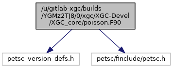
#include "petsc_version_defs.h"
#include <petsc/finclude/petsc.h>

Include dependency graph for poisson.F90:

Data Types
module	f90moduleinterfaces
	Explicit interfaces to somve PETSc function used by the FSA solver. More...
interface	f90moduleinterfaces::pcsetapplicationcontext
interface	f90moduleinterfaces::pcgetapplicationcontext
interface	f90moduleinterfaces::matcreateshell
interface	f90moduleinterfaces::matshellsetcontext
interface	f90moduleinterfaces::matshellgetcontext

Functions/Subroutines
subroutine	init_poisson (pbd0, pbdH, AbdH, psi_center, B_center, den_center, temp_center, f0_dden_center, f0_dtemp_center)
subroutine	pcshermanmorrisonapply (pc, xin, yout, ierr)
	Applies a Sherman-Morrison preconditioner. More...
subroutine	create_2field_solver (grid, bd, solver, solver_data)
	Sets up a 2x2 block solver for the Poisson equation. The first row is the Poisson equation, the second row is a constraint equation for the flux-surface averaged potential. More...
subroutine	make_12mat (grid, Bmat, BIdentMat, FSAMass_Te, solver, bd, scale, xgc_petsc)
subroutine	make_21mat (grid, Cmat, Cio, Bmat, CConstBCVec, bd, xgc_petsc, petsc_xgc_bd)
subroutine	set_rhs_bd_and_sol_bd (rhs, rhs_bd, sol_bd)
subroutine	save_rhs_poisson (xgc_rhs, iflag, ipc)
	Save the charge density for time averaging of the Poisson equation. More...
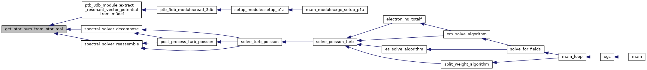
integer function	get_ntor_num_from_ntor_real (ntor_real, nphi, wedge_n)
	Calculates the numerical toroidal mode number for a given real toroidal mode number. More...
subroutine	fourier_filter_n_m_range_parallel_wrap (field_inout, bd_width)
subroutine	fourier_filter_single_n_flex_wrap (field_inout, field_ntor, bd_width)
subroutine	set_petsc_rhs_vec_axisymmetric_poisson (xgc_rhs, xgc_rhs_bd, xgc_sol_bd)
	Places rhs and (optionally) boundary condition data into a PETSc vector. More...
subroutine	set_to_sheath_pot (tmp00_surf)
	Sets initial guess for the iterative axisymmetric poisson solver using the simple00 solver. The initial guess is stored in psnpot0m. More...
subroutine	solve_axisymmetric_poisson_iter (pot0m)
	Poisson solver that uses an iterative method to solve for the axisymmetric electrostatic potential: The Poisson equation for the axisymmetric mode is \[ -\nabla_\perp \cdot \xi \nabla_\perp \overline{\phi}_{k+1} + \frac{e n_0/T_{e,0}} \overline{\phi}_{k+1} = e \left( \langle \overline{\delta n_i} \rangle_g - \overline{\delta n_{e,NA}} \right) + \frac{e n_0/T_{e,0}} \langle \phi_{k} \rangle_{fs} \] where \(k\) is the iteration index, \(xi\) is the electric susceptibility, \(e\) is the elementary charge, \(n_0\) and \(T_0\) are the background density and temperature, \(\langle \overline{\delta n_i} \rangle_g\) is the gyroaveraged ion (gyrocenter) charge density, \(\overline{\delta n_{e,NA}}\) is the non-adiabatic electron charge density, and \(\langle\dots\rangle_{fs}\) is the the flux-surface average. \(\overline{\dots}\) is the toroidal average. More...
subroutine	axisym_mat_mult (A, X, Y, ierr)
	Subroutine used to apply the shell matrix representing the left hand side of the axisymmetric Poisson equation \[ -\nabla_\perp \cdot \xi \nabla_\perp \overline{\phi} + \frac{e n_0/T_{e,0}} \left( \overline{\phi} - \langle \overline{\phi} \rangle_{fs} \right) \] . More...
subroutine	axisym_ad_mat_mult (A, X, Y, ierr)
	Subroutine used to apply the shell matrix representing the adiabatic term in the axisymmetric Poisson equation \[ \frac{e n_0/T_{e,0}} \left( \overline{\phi} - \alpha(\psi) \langle \overline{\phi} \rangle_{fs} \right) \] . More...
subroutine	axisym_pc_apply (pc, X, Y, ierr)
	Subroutine used to apply the shell preconditioner used in the iterative solution of the axisymmetric Poisson equation. More...
subroutine	solve_axisymmetric_poisson_two_step_fsa (xgc_rhs, xgc_rhs00, xgc_rhs_bd, xgc_rhs_bd00, xgc_sol_bd, xgc_sol_bd00, pot0m, dpot)
	Simple two-step 2D solver driver for the axisymmetric potential and one-step solver ("FSA-solver") with constraint equation for the flux-surface averaged potential. For the two-step solver, the RHS is the flux-surface averaged charge density, the LHS consists only of the polarization operator. The result of the 2D solve is flux-surface averaged; i.e., the result is \(\langle\phi\rangle\) The Poisson equation for the flux-surface averaged mode is \[ -\nabla_\perp \cdot \xi \nabla_\perp \overline{\phi} = e \left\langle \left( \langle \overline{\delta n_i} \rangle_g - \overline{\delta n_{e,NA}} \right) \right\rangle_{fs} \] where \(xi\) is the electric susceptibility, \(e\) is the elementary charge, \(n_0\) is the background density, \(\langle \overline{\delta n_i} \rangle_g\) is the gyroaveraged ion (gyrocenter) charge density, \(\overline{\delta n_{e,NA}}\) is the non-adiabatic electron charge density, and \(\langle\dots\rangle_{fs}\) is the the flux-surface average. \(\overline{\dots}\) is the toroidal average. More...
subroutine	positive_phi00_sol (tmp00_surf, pot0m)
subroutine	limit_phi_pert (pot00_2d, temp_ev_elec, pot0m)
	Routine to post process the solution from the axisymmetric poisson solver. More...
subroutine	private_heuristic_pot (pot00_2d, pot0m)
subroutine	set_natural_boundary (pot0m, bc)
subroutine	add_pot0 (pot0m)
subroutine	poisson_turb_petsc_solve (xgc_rhs, xgc_field)
	Routine to solve the non-axisymmetric Poisson equation: \[ -\nabla_\perp \cdot \xi \nabla_\perp \delta\phi + \frac{e n_0/T_{e,0}} \delta\phi = e \left( \langle \delta n_i \rangle_g - \overline{\delta n_{e,NA}} \right) \] . More...
subroutine	poisson_turb_petsc_spectral_solve (xgc_rhs_spectral, xgc_field_spectral)
	Routine to solve the non-axisymmetric Poisson equation: \[ -\nabla_\perp \cdot \xi \nabla_\perp \delta\phi + \frac{e n_0/T_{e,0}} \delta\phi = e \left( \langle \delta n_i \rangle_g - \overline{\delta n_{e,NA}} \right) \] . More...
integer(c_int) function	get_solverh_nbndry ()
integer(c_int) function	get_solver00_nbndry ()
integer(c_int) function	solver00_use_this_rank_int ()
integer(c_int) function	solverh_use_this_rank_int ()
integer(c_int) function	solvera_use_this_rank_int (CV_int)
subroutine	solve_ampere_cv (xgc_rhs, xgc_rhs2, Ah)
subroutine	solve_ampere_cv_spec (xgc_rhs_spectral, xgc_rhs2_spectral, xgc_field_spectral)
subroutine	solve_ampere (xgc_rhs, xgc_rhs2, Ah)
subroutine	solve_ampere_spec (xgc_rhs_spectral, xgc_rhs2_spectral, xgc_field_spectral)
subroutine	ptb_3db_damping_factor_em_wrap ()
subroutine	save_ah ()
subroutine	backup_ptb_3db_rampup_fac ()
subroutine	apply_radial_hyperviscosity (input, output)
subroutine	add_as_vac (As, dt)
subroutine	subtract_as_vac (As)
subroutine	cce_send_receive_as_wrap ()

Function/Subroutine Documentation

subroutine add_as_vac	(	real(8), dimension(grid_global%nnode)	As,
		real(8), intent(in)	dt
	)

subroutine add_pot0

(

real(8), dimension(grid%nnode)

pot0m

)

Here is the call graph for this function:

Here is the caller graph for this function:

subroutine apply_radial_hyperviscosity	(	real(8), dimension(grid_global%nnode)	input,
		real(8), dimension(grid_global%nnode)	output
	)

Here is the call graph for this function:

Here is the caller graph for this function:

subroutine axisym_ad_mat_mult	(		A,
			X,
			Y,
			ierr
	)

Subroutine used to apply the shell matrix representing the adiabatic term in the axisymmetric Poisson equation

\[ \frac{e n_0/T_{e,0}} \left( \overline{\phi} - \alpha(\psi) \langle \overline{\phi} \rangle_{fs} \right) \]

.

Parameters

[in]	A	Shell matrix which multiplies X, Petsc Mat
[in]	X	Vector to be multiplied, Petsc Vec
[out]	Y	Vector to store product A*X, Petsc Vec
[out]	ierr	PETSc Error code

Here is the call graph for this function:

Here is the caller graph for this function:

subroutine axisym_mat_mult	(		A,
			X,
			Y,
			ierr
	)

Subroutine used to apply the shell matrix representing the left hand side of the axisymmetric Poisson equation

\[ -\nabla_\perp \cdot \xi \nabla_\perp \overline{\phi} + \frac{e n_0/T_{e,0}} \left( \overline{\phi} - \langle \overline{\phi} \rangle_{fs} \right) \]

.

Parameters

[in]	A	Shell matrix which multiplies X, Petsc Mat
[in]	X	Vector to be multiplied, Petsc Vec
[out]	Y	Vector to store product A*X, Petsc Vec
[out]	ierr	PETSc Error code

Here is the call graph for this function:

Here is the caller graph for this function:

subroutine axisym_pc_apply	(		pc,
			X,
			Y,
			ierr
	)

Subroutine used to apply the shell preconditioner used in the iterative solution of the axisymmetric Poisson equation.

Parameters

[in]	pc	Shell preconditioner which is applied to residual X, Petsc PC
[in]	X	Residual vector, Petsc Vec
[out]	Y	Preconditioned residual vector, Petsc Vec
[out]	ierr	PETSc Error code

Here is the call graph for this function:

Here is the caller graph for this function:

subroutine backup_ptb_3db_rampup_fac

(

)

Here is the caller graph for this function:

subroutine cce_send_receive_as_wrap

(

)

Here is the call graph for this function:

Here is the caller graph for this function:

subroutine create_2field_solver	(	type(grid_type)	grid,
		integer, dimension(grid%nnode)	bd,
		type(xgc_solver)	solver,
		type(solver_init_data), intent(in)	solver_data
	)

Sets up a 2x2 block solver for the Poisson equation. The first row is the Poisson equation, the second row is a constraint equation for the flux-surface averaged potential.

Parameters

[in]	grid	XGC grid object, type(grid_type)
[in]	bd	Solver boundary mask, 1 if not in boundary vertex list
[in,out]	solver	XGC solver object into which to put the new solver, type(xgc_solver)
[in]	solver_data	Data needed for settug up the ssolver, type(solver_init_data)

Here is the call graph for this function:

Here is the caller graph for this function:

subroutine fourier_filter_n_m_range_parallel_wrap	(	real(kind=8), dimension(grid_global%nnode), intent(inout)	field_inout,
		real(kind=8)	bd_width
	)

Here is the call graph for this function:

Here is the caller graph for this function:

subroutine fourier_filter_single_n_flex_wrap	(	real(kind=8), dimension(grid_global%nnode), intent(inout)	field_inout,
		real(kind=8), dimension(grid_global%nnode,2), intent(out)	field_ntor,
		real(kind=8)	bd_width
	)

Here is the call graph for this function:

Here is the caller graph for this function:

integer function get_ntor_num_from_ntor_real	(	integer, intent(in)	ntor_real,
		integer, intent(in)	nphi,
		integer, intent(in)	wedge_n
	)

Calculates the numerical toroidal mode number for a given real toroidal mode number.

Parameters

[in]	ntor_real	Real toroidal mode number, integer
[in]	nphi	Number of toroidal planes per wedge, integer
[in]	wedge_n	Number of wedges per toroidal circuit, integer

Here is the call graph for this function:

Here is the caller graph for this function:

integer(c_int) function get_solver00_nbndry

(

)

Here is the call graph for this function:

Here is the caller graph for this function:

integer(c_int) function get_solverh_nbndry

(

)

subroutine init_poisson	(	integer, dimension(grid%nnode)	pbd0,
		integer, dimension(grid%nnode)	pbdH,
		integer, dimension(grid%nnode)	AbdH,
		real(8), dimension(grid%ntriangle)	psi_center,
		real(8), dimension(grid%ntriangle, 3)	B_center,
		real(8), dimension(grid%ntriangle, 0:ptl_nsp)	den_center,
		real(8), dimension(grid%ntriangle, 0:ptl_nsp)	temp_center,
		real(8), dimension(grid%ntriangle, 0:ptl_nsp)	f0_dden_center,
		real(8), dimension(grid%ntriangle, 0:ptl_nsp)	f0_dtemp_center
	)

Here is the call graph for this function:

Here is the caller graph for this function:

subroutine limit_phi_pert	(	real (8), dimension(grid%nnode)	pot00_2d,
		real(8), dimension(grid%nnode), intent(in)	temp_ev_elec,
		real(8), dimension(grid%nnode)	pot0m
	)

Routine to post process the solution from the axisymmetric poisson solver.

Parameters

[in]	grid	XGC grid data object
[in,out]	psn	XGC field data object

Here is the call graph for this function:

Here is the caller graph for this function:

subroutine make_12mat	(	type(grid_type)	grid,
		intent(inout)	Bmat,
			BIdentMat,
		intent(in)	FSAMass_Te,
		type(xgc_solver)	solver,
		integer, dimension(grid%nnode), intent(in)	bd,
		real (8), intent(in)	scale,
		dimension(grid%nnode), intent(in)	xgc_petsc
	)

Here is the call graph for this function:

Here is the caller graph for this function:

subroutine make_21mat	(	type(grid_type)	grid,
			Cmat,
			Cio,
		intent(in)	Bmat,
			CConstBCVec,
		integer, dimension(grid%nnode), intent(in)	bd,
		dimension(grid%nnode), intent(in)	xgc_petsc,
		dimension(grid%nnode), intent(in)	petsc_xgc_bd
	)

Here is the caller graph for this function:

subroutine pcshermanmorrisonapply	(		pc,
			xin,
			yout,
			ierr
	)

Applies a Sherman-Morrison preconditioner.

Parameters

[in,out]	pc	PETCs PC object (manages preconditioners)
	xin	???, Vec
	yout	???, Vec
[out]	ierr	PETc error code

Here is the caller graph for this function:

subroutine poisson_turb_petsc_solve	(	real (8), dimension(grid%nnode)	xgc_rhs,
		real (8), dimension(grid%nnode)	xgc_field
	)

Routine to solve the non-axisymmetric Poisson equation:

\[ -\nabla_\perp \cdot \xi \nabla_\perp \delta\phi + \frac{e n_0/T_{e,0}} \delta\phi = e \left( \langle \delta n_i \rangle_g - \overline{\delta n_{e,NA}} \right) \]

.

Parameters

[in]	grid	XGC grid data object
[in,out]	psn	XGC field data object

Here is the call graph for this function:

Here is the caller graph for this function:

subroutine poisson_turb_petsc_spectral_solve	(	real (8), dimension(grid%nnode,2)	xgc_rhs_spectral,
		real (8), dimension(grid%nnode,2)	xgc_field_spectral
	)

Routine to solve the non-axisymmetric Poisson equation:

\[ -\nabla_\perp \cdot \xi \nabla_\perp \delta\phi + \frac{e n_0/T_{e,0}} \delta\phi = e \left( \langle \delta n_i \rangle_g - \overline{\delta n_{e,NA}} \right) \]

.

Parameters

[in]	grid	XGC grid data object
[in,out]	psn	XGC field data object

Here is the call graph for this function:

Here is the caller graph for this function:

subroutine positive_phi00_sol	(	real (kind=8), dimension(grid%npsi_surf)	tmp00_surf,
		real(8), dimension(grid%nnode)	pot0m
	)

Here is the call graph for this function:

Here is the caller graph for this function:

subroutine private_heuristic_pot	(	real (8), dimension(grid%nnode)	pot00_2d,
		real(8), dimension(grid%nnode)	pot0m
	)

Here is the call graph for this function:

Here is the caller graph for this function:

subroutine ptb_3db_damping_factor_em_wrap

(

)

Here is the call graph for this function:

Here is the caller graph for this function:

subroutine save_ah

(

)

subroutine save_rhs_poisson	(	real(8), dimension(grid%nnode)	xgc_rhs,
		integer(c_int)	iflag,
		integer(c_int)	ipc
	)

Save the charge density for time averaging of the Poisson equation.

Parameters

[in]	grid	XGC grid data structure, type(grid_type)
[in,out]	psn	XGC field data structure, type(psn_type)
[in,out]	solver	XGC solver object, type(xgc_solver)
[in]	iflag	Adiabatic solve indicator, integer
[in]	ipc	RK2 stage index, integer
[out]	do_solve_poisson	Whether to solve Ampere's law after saving RHS, logical

Here is the caller graph for this function:

subroutine set_natural_boundary	(	real(8), dimension(grid%nnode)	pot0m,
		integer, dimension(grid%nnode)	bc
	)

Here is the caller graph for this function:

subroutine set_petsc_rhs_vec_axisymmetric_poisson	(	real(8), dimension(grid%nnode)	xgc_rhs,
		real(8), dimension(psn%solver00%n_boundary)	xgc_rhs_bd,
		real(8), dimension(psn%solver00%n_boundary)	xgc_sol_bd
	)

Places rhs and (optionally) boundary condition data into a PETSc vector.

Parameters

[in]	grid	Solver grid data, type(grid_type)
[in,out]	psn	Field data; the rhs XGC data is stored there, type(psn_type)
[in,out]	solver	XGC solver object; the rhs PETSc vector is stored there, type(xgc_solver)

Here is the call graph for this function:

subroutine set_rhs_bd_and_sol_bd	(	real (8), dimension(grid%nnode)	rhs,
		real (8), dimension(psn%solver00%n_boundary)	rhs_bd,
		real (8), dimension(psn%solver00%n_boundary)	sol_bd
	)

Here is the call graph for this function:

Here is the caller graph for this function:

subroutine set_to_sheath_pot

(

real (8), dimension(grid%npsi_surf)

tmp00_surf

)

Sets initial guess for the iterative axisymmetric poisson solver using the simple00 solver. The initial guess is stored in psnpot0m.

Parameters

[in]	grid	Solver grid data, type(grid_type)
[in,out]	psn	Field data; the pot0m is stored there, type(psn_type)

Here is the call graph for this function:

Here is the caller graph for this function:

subroutine solve_ampere	(	real (8), dimension(grid%nnode)	xgc_rhs,
		real (8), dimension(grid%nnode)	xgc_rhs2,
		real (8), dimension(grid%nnode), intent(out)	Ah
	)

Here is the call graph for this function:

Here is the caller graph for this function:

subroutine solve_ampere_cv	(	real (8), dimension(grid%nnode)	xgc_rhs,
		real (8), dimension(grid%nnode)	xgc_rhs2,
		real (8), dimension(grid%nnode), intent(out)	Ah
	)

Here is the call graph for this function:

Here is the caller graph for this function:

subroutine solve_ampere_cv_spec	(	real (8), dimension(grid%nnode,2)	xgc_rhs_spectral,
		real (8), dimension(grid%nnode,2)	xgc_rhs2_spectral,
		real (8), dimension(grid%nnode,2)	xgc_field_spectral
	)

Here is the call graph for this function:

Here is the caller graph for this function:

subroutine solve_ampere_spec	(	real (8), dimension(grid%nnode,2)	xgc_rhs_spectral,
		real (8), dimension(grid%nnode,2)	xgc_rhs2_spectral,
		real (8), dimension(grid%nnode,2)	xgc_field_spectral
	)

Here is the call graph for this function:

Here is the caller graph for this function:

subroutine solve_axisymmetric_poisson_iter

(

real(8), dimension(grid%nnode)

pot0m

)

Poisson solver that uses an iterative method to solve for the axisymmetric electrostatic potential: The Poisson equation for the axisymmetric mode is

\[ -\nabla_\perp \cdot \xi \nabla_\perp \overline{\phi}_{k+1} + \frac{e n_0/T_{e,0}} \overline{\phi}_{k+1} = e \left( \langle \overline{\delta n_i} \rangle_g - \overline{\delta n_{e,NA}} \right) + \frac{e n_0/T_{e,0}} \langle \phi_{k} \rangle_{fs} \]

where \(k\) is the iteration index, \(xi\) is the electric susceptibility, \(e\) is the elementary charge, \(n_0\) and \(T_0\) are the background density and temperature, \(\langle \overline{\delta n_i} \rangle_g\) is the gyroaveraged ion (gyrocenter) charge density, \(\overline{\delta n_{e,NA}}\) is the non-adiabatic electron charge density, and \(\langle\dots\rangle_{fs}\) is the the flux-surface average. \(\overline{\dots}\) is the toroidal average.

The RHS and LHS of the axisymmetric equation can be Fourier-filtered (poloidal modes). The LHS of the non-axisymmetric equation can be Fourier-filtered in the toroidal and poloidal direction. The solver in both cases is a linear finite-element solver on an unstructured triangular grid.

Parameters

[in]	grid	Solver grid data, type(grid_type)
[in,out]	psn	Field data; the potential is stored there, type(psn_type)

Here is the call graph for this function:

subroutine solve_axisymmetric_poisson_two_step_fsa	(	real (8), dimension(grid%nnode)	xgc_rhs,
		real (8), dimension(grid%nnode)	xgc_rhs00,
		real (8), dimension(psn%solverh%n_boundary)	xgc_rhs_bd,
		real (8), dimension(psn%solver00%n_boundary)	xgc_rhs_bd00,
		real (8), dimension(psn%solverh%n_boundary)	xgc_sol_bd,
		real (8), dimension(psn%solver00%n_boundary)	xgc_sol_bd00,
		real(8), dimension(grid%nnode)	pot0m,
		real(8), dimension(grid%nnode)	dpot
	)

Simple two-step 2D solver driver for the axisymmetric potential and one-step solver ("FSA-solver") with constraint equation for the flux-surface averaged potential. For the two-step solver, the RHS is the flux-surface averaged charge density, the LHS consists only of the polarization operator. The result of the 2D solve is flux-surface averaged; i.e., the result is \(\langle\phi\rangle\) The Poisson equation for the flux-surface averaged mode is

\[ -\nabla_\perp \cdot \xi \nabla_\perp \overline{\phi} = e \left\langle \left( \langle \overline{\delta n_i} \rangle_g - \overline{\delta n_{e,NA}} \right) \right\rangle_{fs} \]

where \(xi\) is the electric susceptibility, \(e\) is the elementary charge, \(n_0\) is the background density, \(\langle \overline{\delta n_i} \rangle_g\) is the gyroaveraged ion (gyrocenter) charge density, \(\overline{\delta n_{e,NA}}\) is the non-adiabatic electron charge density, and \(\langle\dots\rangle_{fs}\) is the the flux-surface average. \(\overline{\dots}\) is the toroidal average.

NOTE: The two-step solver does not support non-zero Dirichlet boundary conditions!

The FSA solver solves the same equation as the outer-iterative solver (solve_axisymmetric_poisson_iter), but with a twist. The flux-surface averaged potential is treated as an independent field \(\lambda\) in the Poisson equation. In order to make the equation consistent, a second (constraint) equation is added that enforces \(\lambda=\langle\phi\rangle_{fs}\). So the FSA solver solves a 2x2 block system.

Parameters

[in]	grid	Solver grid data, type(grid_type)
[in,out]	psn	Field data; the potential is stored there, type(psn_type)

Here is the call graph for this function:

Here is the caller graph for this function:

integer(c_int) function solver00_use_this_rank_int

(

)

Here is the call graph for this function:

Here is the caller graph for this function:

integer(c_int) function solvera_use_this_rank_int

(

integer(c_int)

CV_int

)

integer(c_int) function solverh_use_this_rank_int

(

)

subroutine subtract_as_vac

(

real(8), dimension(grid_global%nnode)

As

)