#include <petsc/finclude/petsc.h>#include <petsc/finclude/petscts.h>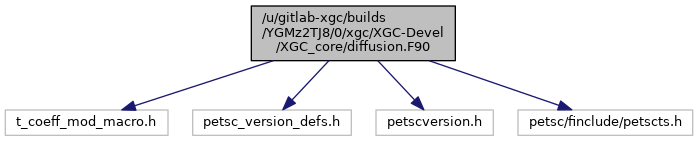
Functions/Subroutines | |
| subroutine | ts_init (a_bc, a_ts, is_update) |
| Initializes the PETSc time stepper for the 2D diffusion solver. This routine sets up a system of conserving Fick's law type equations on the 2D XGC solver mesh for: density, flow and parallel and perpendicular temperature, i.e., 3*n_species+1 equations. The linear terms of the form \(\nabla \cdot \boldsymbol{D}.\nabla X \) are discretized with linear finite elements. The nonlinear terms are discretized with finite difference. The diffusivity tensor is set up such that only trnasport perpendicular to flux-surfaces is computed by this model. More... | |
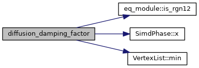
| real(kind=8) function | diffusion_damping_factor (x, psi) |
| Calculates the damping factor for the diffusion coefficients and pinch velocity. More... | |
| real(kind=8) function | diffusion_pol_peak_factor (x) |
| Calculates the poloidal envelope of the anomalous transport By default, anomalous transport is a flux-function similar to 1D transport models. A ballooning structure can be added through the ballooning angle and the ballooning factor. More... | |
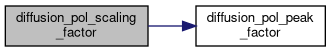
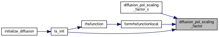
| real(kind=8) function | diffusion_pol_scaling_factor (x) |
| Returns the poloidal transport scaling factor used in the diffusion model. This includes the switch between constant and ballooned transport. More... | |
| real(c_double) function | diffusion_pol_scaling_factor_c (r, z) |
| C interface for the poloidal transport scaling factor. More... | |
| real(kind=8) function | divertor_damping_factor (r, z) |
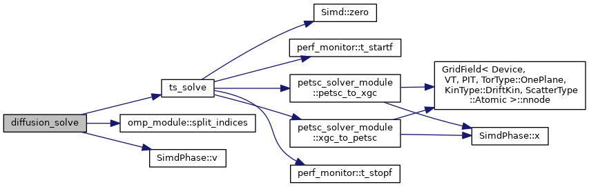
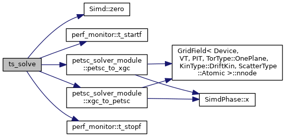
| subroutine | ts_solve (a_ts, a_dt, XX_in, blocksize) |
| This routine performs the actual time integration of the 2D diffusion model. More... | |
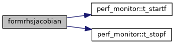
| subroutine | formrhsjacobian (ts, t_dummy, a_XX, J, Jpre, a_ts, ierr) |
| Update the RHS Jacobian In case the RHS Jacobian has any time dependent terms, this routine would compute the time dependent terms and put them into the final Jacobian for the present stage/step. More... | |
| subroutine | formrhsjacobianlocal (a_ts, Jpre, XX_in, nn, ierr) |
| Helper routine in XGC space for setting up the non-linear terms of the RHS Jacobian. This routine is used to compute any time dependent terms on the XGC solver grid. The result of this calculation will be inserted in the final RHS Jacobian. More... | |
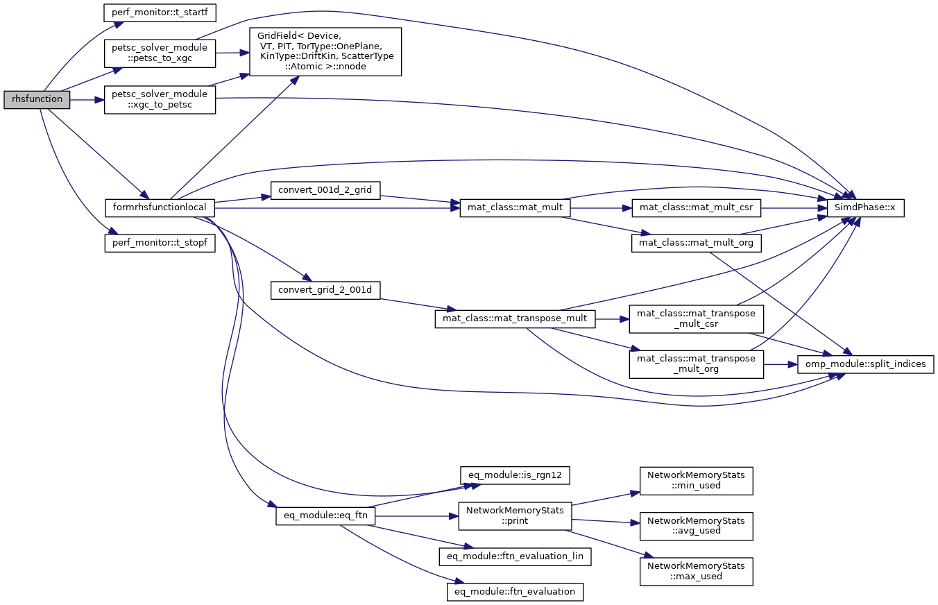
| subroutine | rhsfunction (ts, time, a_XX, a_FF, a_ts, ierr) |
| Evaluates the RHS equation. More... | |
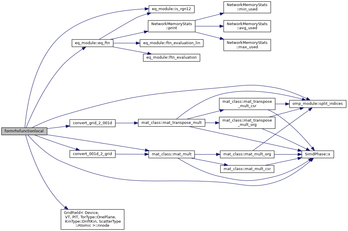
| subroutine | formrhsfunctionlocal (a_ts, time, ts_it, snes_it, XX_in, div_gamma_in, rhs_out, nn) |
| Computations in XGC space for RHS evaluation This includes 4 nonlinear terms for each species, one in the momentum equation, and three in the temperature equation. The terms are: (1/n) grad(n).(D+eta).grad(u) = (1/n) (D+eta) (dn/dr)(du/dr) in the momentum equation, and (T/n) div(D.grad(n)) = (T/n) d(D dn/dr)/dr (1/3n) grad(n).(5D+2chi).grad(T) = (5D+2chi)/(3n) (dn/dr)(dT/dr) (2m/3) grad(u).eta.grad(u) = (2m eta)/3 (du/dr)^2 Since this involves only radial gradients, we can simply use the XGC matrix gridgradientx. We have to take care, though, that vertices with undefined grad(psi) do not contribute (since we defined the tensor diffusivity to be D_ij=D(psi) psi_hat psi_hat). More... | |
| subroutine | set_diffusion_pol_peak_fsa_norm_ptr (nnode, pol_peak_fsa_norm_in) |
| Set the Fortran pointer to the C++-owned poloidal peaking normalization. More... | |
| subroutine | diffusion_solve (nn, XX_in, dt) |
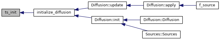
| subroutine | initialize_diffusion (bd, is_update) |
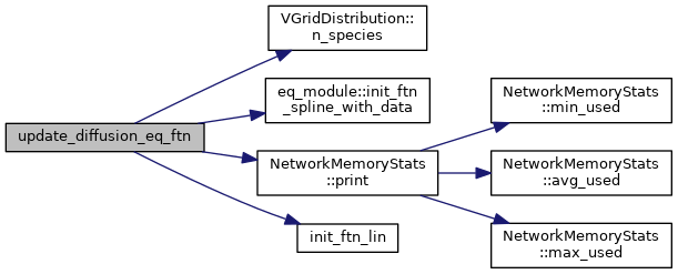
| subroutine | update_diffusion_eq_ftn (n_species, npsi_in, psi_in, diff_coeff_in) |
Function/Subroutine Documentation
◆ diffusion_damping_factor()
| real(kind=8) function diffusion_damping_factor | ( | real (kind=8), dimension(2), intent(in) | x, |
| real (kind=8), intent(in) | psi | ||
| ) |
Calculates the damping factor for the diffusion coefficients and pinch velocity.
- Parameters
-
[in] x Input (R,Z) coordinates, real(8) [in] psi Input poloidal magnetic flux, real(8)

◆ diffusion_pol_peak_factor()
| real (kind=8) function diffusion_pol_peak_factor | ( | real (kind=8), dimension(2), intent(in) | x | ) |
Calculates the poloidal envelope of the anomalous transport By default, anomalous transport is a flux-function similar to 1D transport models. A ballooning structure can be added through the ballooning angle and the ballooning factor.
- Parameters
-
[in] x Input (R,Z) coordinates, real(8)

◆ diffusion_pol_scaling_factor()
| real (kind=8) function diffusion_pol_scaling_factor | ( | real (kind=8), dimension(2), intent(in) | x | ) |
Returns the poloidal transport scaling factor used in the diffusion model. This includes the switch between constant and ballooned transport.
- Parameters
-
[in] x Input (R,Z) coordinates, real(8)
◆ diffusion_pol_scaling_factor_c()
| real(c_double) function diffusion_pol_scaling_factor_c | ( | real(c_double), intent(in), value | r, |
| real(c_double), intent(in), value | z | ||
| ) |
C interface for the poloidal transport scaling factor.
- Parameters
-
[in] r Major radius, real(8) [in] z Vertical coordinate, real(8)

◆ diffusion_solve()
| subroutine diffusion_solve | ( | integer, intent(in), value | nn, |
| real (8), dimension(nn,diff_timestepper%blocksize) | XX_in, | ||
| real(8), intent(in), value | dt | ||
| ) |
◆ divertor_damping_factor()
| real(kind=8) function divertor_damping_factor | ( | real (8) | r, |
| real (8) | z | ||
| ) |

◆ formrhsfunctionlocal()
| subroutine formrhsfunctionlocal | ( | type(xgc_ts) | a_ts, |
| time, | |||
| ts_it, | |||
| snes_it, | |||
| real (kind=8), dimension(nn,a_ts%blocksize), intent(in) | XX_in, | ||
| real (kind=8), dimension(nn), intent(in) | div_gamma_in, | ||
| real (kind=8), dimension(nn,a_ts%blocksize), intent(out) | rhs_out, | ||
| integer | nn | ||
| ) |
Computations in XGC space for RHS evaluation This includes 4 nonlinear terms for each species, one in the momentum equation, and three in the temperature equation. The terms are: (1/n) grad(n).(D+eta).grad(u) = (1/n) (D+eta) (dn/dr)(du/dr) in the momentum equation, and (T/n) div(D.grad(n)) = (T/n) d(D dn/dr)/dr (1/3n) grad(n).(5D+2chi).grad(T) = (5D+2chi)/(3n) (dn/dr)(dT/dr) (2m/3) grad(u).eta.grad(u) = (2m eta)/3 (du/dr)^2 Since this involves only radial gradients, we can simply use the XGC matrix gridgradientx. We have to take care, though, that vertices with undefined grad(psi) do not contribute (since we defined the tensor diffusivity to be D_ij=D(psi) psi_hat psi_hat).
- Parameters
-
[in,out] ts PETSc time stepping object, TS [in] time Time stamp, PETScReal, PETScReal [in] ts_it TS time step index, PETScInt [in] snes_it SNES iteration index, PETScInt [in] XX_in Input quantities [n,ui,Tipa,Tipe,{ue,Tepa,Tepe}], real(8) [in] div_gamma_in div(D.grad(n)-n*v_pinch) [out] rhs_out Nonlinear RHS terms [n,ui,Tipa,Tipe,{ue,Tepa,Tepe}], real(8) [in] nn Number of mesh vertices, integer

◆ formrhsjacobian()
| subroutine formrhsjacobian | ( | ts, | |
| t_dummy, | |||
| a_XX, | |||
| J, | |||
| Jpre, | |||
| type(xgc_ts) | a_ts, | ||
| intent(out) | ierr | ||
| ) |
Update the RHS Jacobian In case the RHS Jacobian has any time dependent terms, this routine would compute the time dependent terms and put them into the final Jacobian for the present stage/step.
- Parameters
-
[in] ts PETSc time stepping object, TS [in] t_dummy Time stamp, PETScReal [in] a_XX Current fields, Vec [in,out] J Jacobian, Mat [in,out] Jpre Preconditioned Jacobian, Mat [in,out] a_ts XGC time stepping object, type(xgc_ts) [out] ierr Error code, PETScErrorCode

◆ formrhsjacobianlocal()
| subroutine formrhsjacobianlocal | ( | type(xgc_ts), intent(inout) | a_ts, |
| intent(inout) | Jpre, | ||
| real (kind=8), dimension(nn,a_ts%blocksize), intent(in) | XX_in, | ||
| integer | nn, | ||
| intent(inout) | ierr | ||
| ) |
Helper routine in XGC space for setting up the non-linear terms of the RHS Jacobian. This routine is used to compute any time dependent terms on the XGC solver grid. The result of this calculation will be inserted in the final RHS Jacobian.
- Parameters
-
[in,out] a_ts type(xgc_ts), XGC ts_object with grid information, etc. [in,out] Jpre PETSc Mat, the RHS Jacobian matrix [in] n real(8), perturbed electron density [in] ui real(8), A_parallel [in] Ti real(8), electrostatic potential [in] ue real(8), del^2(A_parallel) [in] Te real(8), del^2(A_parallel) [in] nn integer, mesh size [in,out] ierr PetscErrorCode
◆ initialize_diffusion()
| subroutine initialize_diffusion | ( | integer, dimension(grid_global%nnode), intent(in) | bd, |
| integer, intent(in), value | is_update | ||
| ) |
◆ rhsfunction()
| subroutine rhsfunction | ( | ts, | |
| time, | |||
| a_XX, | |||
| a_FF, | |||
| type(xgc_ts) | a_ts, | ||
| intent(out) | ierr | ||
| ) |
Evaluates the RHS equation.
- Parameters
-
[in,out] ts PETSc time stepping object, TS [in] time Time stamp, PETScReal [in] a_XX Current field data, Vec [out] a_FF RHS result vecgtor, Vec [in,out] a_ts XGC time stepping object, xgc_ts [in,out] ierr PETScErrorCode

◆ set_diffusion_pol_peak_fsa_norm_ptr()
| subroutine set_diffusion_pol_peak_fsa_norm_ptr | ( | integer(c_int), intent(in), value | nnode, |
| real(c_double), dimension(nnode), intent(in), target | pol_peak_fsa_norm_in | ||
| ) |
Set the Fortran pointer to the C++-owned poloidal peaking normalization.
- Parameters
-
[in] nnode Number of mesh vertices [in] pol_peak_fsa_norm_in Vertex-wise normalized peaking factor
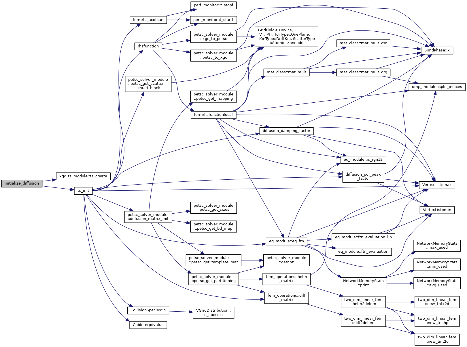
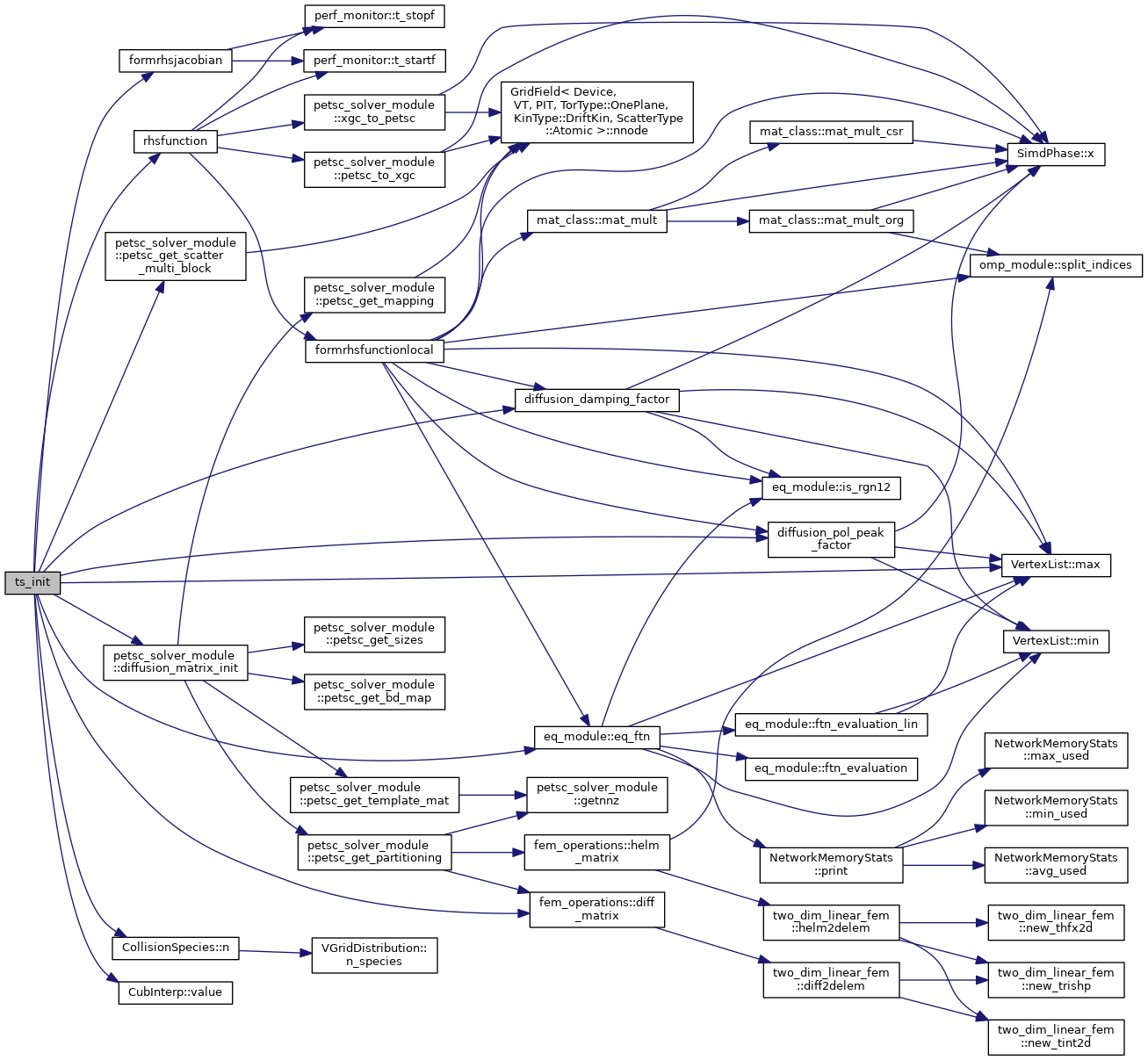
◆ ts_init()
| subroutine ts_init | ( | integer, dimension(grid_global%nnode), intent(in) | a_bc, |
| type(xgc_ts) | a_ts, | ||
| logical, intent(in) | is_update | ||
| ) |
Initializes the PETSc time stepper for the 2D diffusion solver. This routine sets up a system of conserving Fick's law type equations on the 2D XGC solver mesh for: density, flow and parallel and perpendicular temperature, i.e., 3*n_species+1 equations. The linear terms of the form \(\nabla \cdot \boldsymbol{D}.\nabla X \) are discretized with linear finite elements. The nonlinear terms are discretized with finite difference. The diffusivity tensor is set up such that only trnasport perpendicular to flux-surfaces is computed by this model.
- Parameters
-
[in] a_bc Boundary vertices for solver [in,out] a_ts XGC time-stepper structure, type(xgc_ts)
◆ ts_solve()
| subroutine ts_solve | ( | type(xgc_ts), intent(inout) | a_ts, |
| real(kind=8), intent(in) | a_dt, | ||
| real(kind=8), dimension(a_ts%nnode,blocksize), intent(inout) | XX_in, | ||
| intent(in) | blocksize | ||
| ) |
This routine performs the actual time integration of the 2D diffusion model.
- Parameters
-
[in,out] a_ts XGC time-stepper structure, type(xgc_ts) [in] a_dt Time step, real8 [in,out] XX_in Input moments (density, etc.), real8 [in] blocksize Number of equations, integer

◆ update_diffusion_eq_ftn()
| subroutine update_diffusion_eq_ftn | ( | integer, intent(in), value | n_species, |
| integer, intent(in), value | npsi_in, | ||
| real (kind=8), dimension(npsi_in), intent(in) | psi_in, | ||
| real (kind=8), dimension(npsi_in,0:n_species-1,4), intent(in) | diff_coeff_in | ||
| ) |